Systems - 5ESB0

5ESB0 Systems

• Area: Signals and Systems
• Topics: Complex Numbers · Differential Equations · Fourier Transform · Laplace Transform · Transfer Functions and Frequency Response · Feedback and Stability · Controller Design
• Related courses: Signals II (DSP Fundamentals) - 5ESC0 · Control Systems - 5ESD0 · Calculus - 2WBB0
• Notes by a friend: Systems (friend) - 5ESB0

Dynamic systems (theory)
Transfer functions
Laplace transform
Dynamic responses of linear systems
Second order systems
Fourier Transforms
System interconnections and stability
Feedback and feedforward
Feedback controllers (PID)

Laplace Transform (friend) - 5ESC0
Fourier Analysis (friend) - 5ESC0

Transfer Functions

Topic: Transfer Functions and Frequency Response

• Differential system:
  • → normalized
  • Find
  • Parameterize
  • Write boundary conditions: etc…
  • Find as a function of
  • Solve homogeneous differential equation with of form to find
  • Substitute and

Transfer functions H(s) describes the particular solution as an s-dependent amplification of input signal
when → first order
when → second order

• Convolution system:
  • Convolution Integral:
  • Draw a representation of the signals
  • Choose which signal to flip and draw the flipped signal
  • Find all cases and their respective time intervals
  • Find the limits of the convolution integral for each case
  • Compute the convolution integral for each case
  • Express final answer as a piecewise function

→ impulse response | → step response
and
Causality: for
1 when and 0 when step signal → notation:
1 when and 0 impulse signal

• System output summery:
  1. Decompose in terms → | transfer function
  2. Decompose in piecewise constant terms → | impulse response

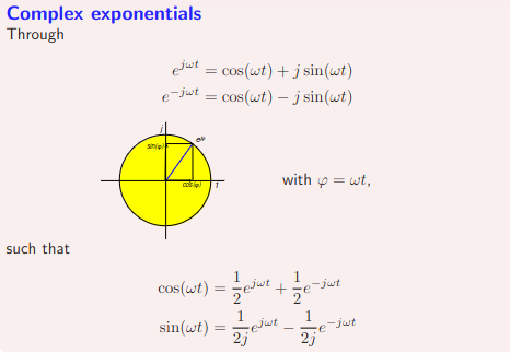
Extra: Complex Exponentials

Topic: Complex Numbers

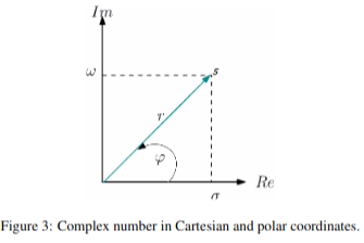
complex number s:
cartesian coord:
polar coord:

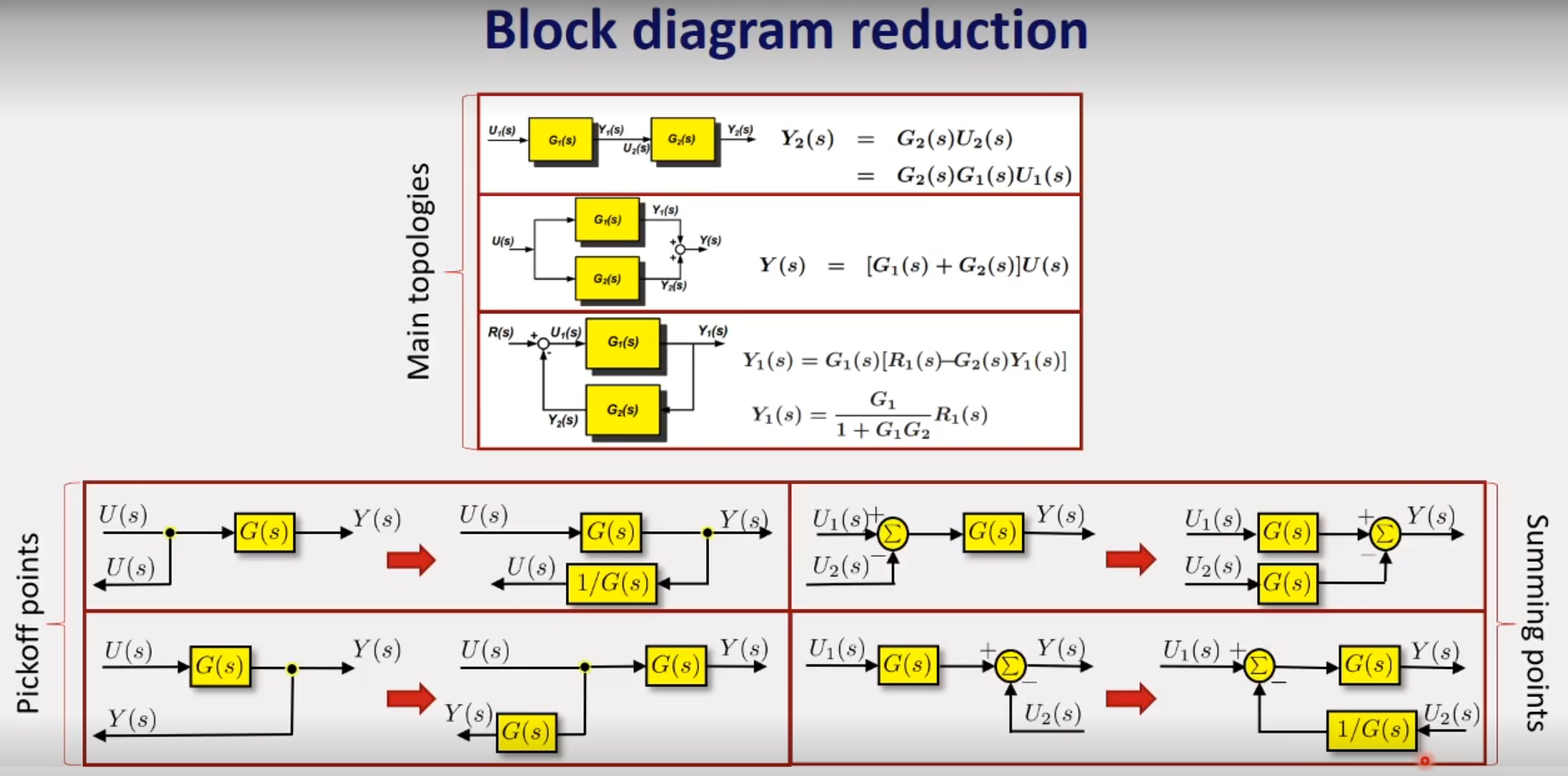
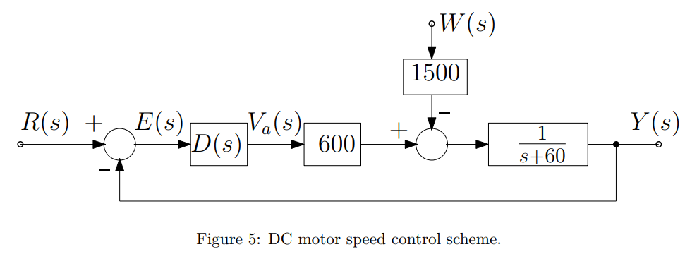
Block Diagrams

e1a7408acfaa5b79f0b3147e84d93bdd_MIT2_04AS13_Lecture10.pdf

Laplace Transform

Topic: Laplace Transform
Relation between and

Laplace Derivation

Substitute

so: for

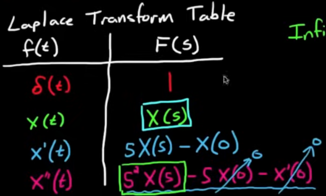
⇒ differentiation | ⇒ integration (use table)

Laplace Differentiation Property

⇒ Basic
⇒ General

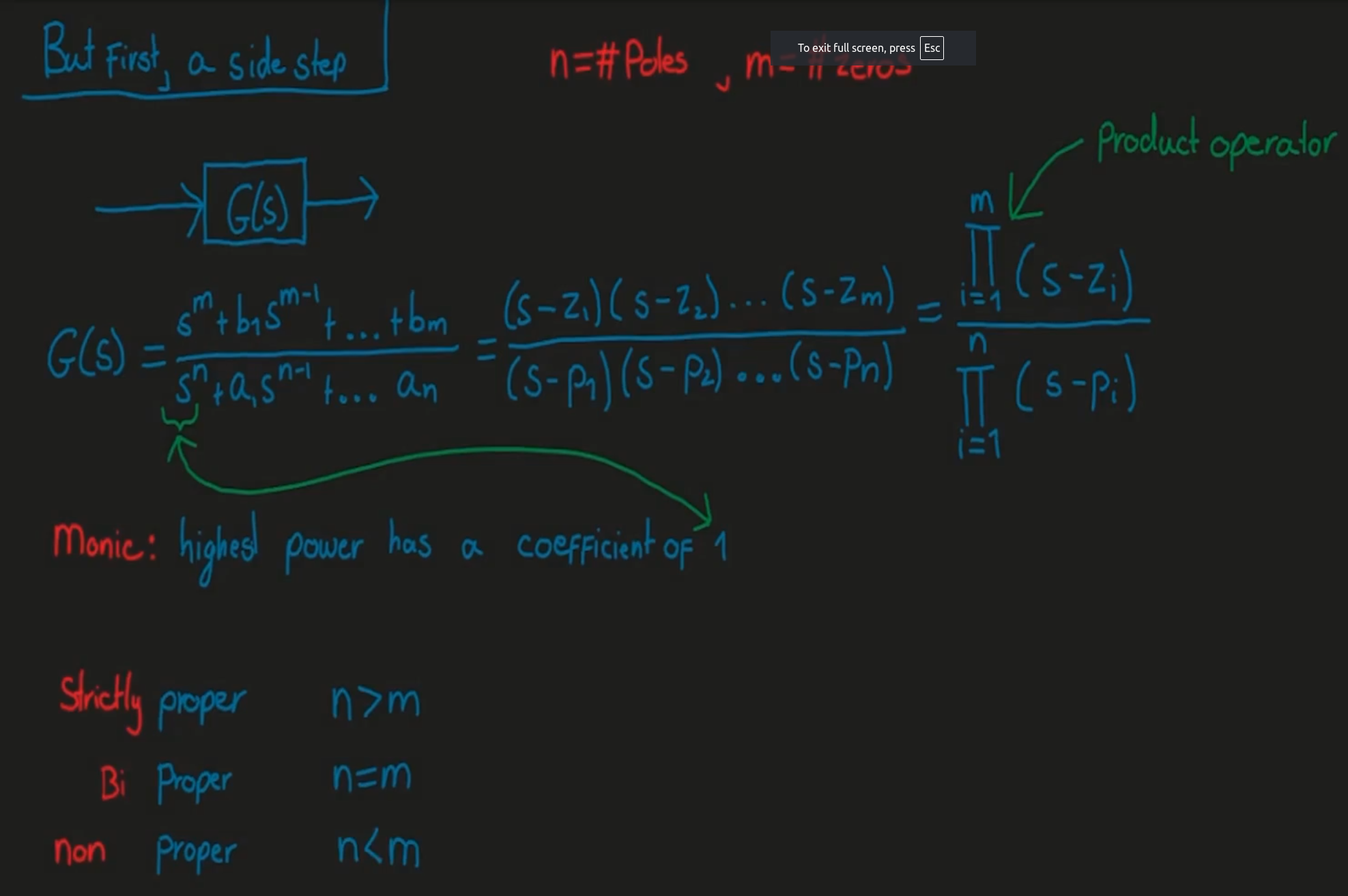
A strictly proper transfer function is a transfer function where the degree of the numerator is less than the degree of the denominator.

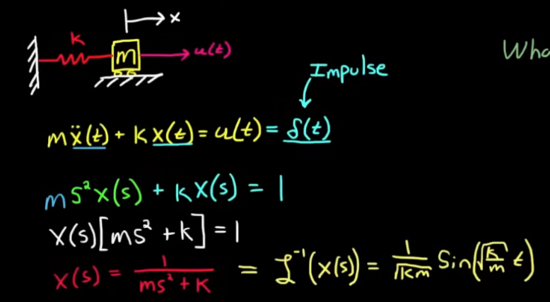
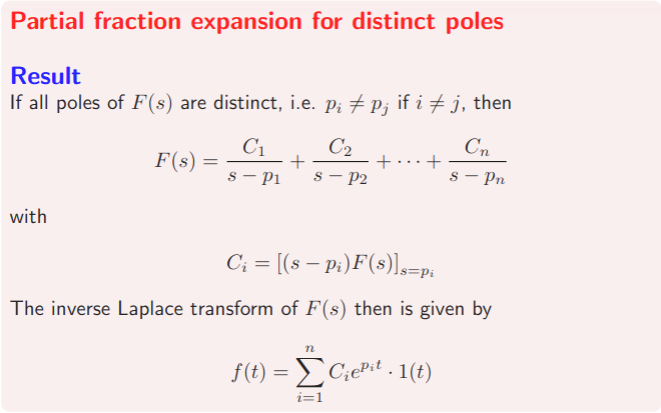
Inverse Laplace Transform:

Dynamic Responses of Linear Systems

Topic: Differential Equations

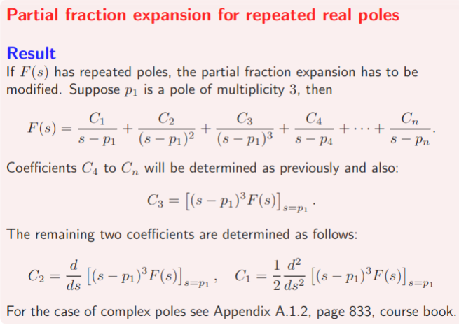
Poles and zeros of come in complex conjugate pairs damping and (undamped) natural frequency.

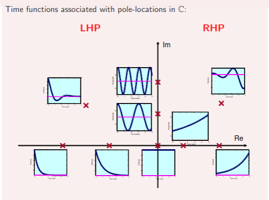
Poles determine the natural (unforced) response of the system
Zeros determine the input signals that do not reach through to the output
If then has zeros in infinity → unstable

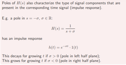
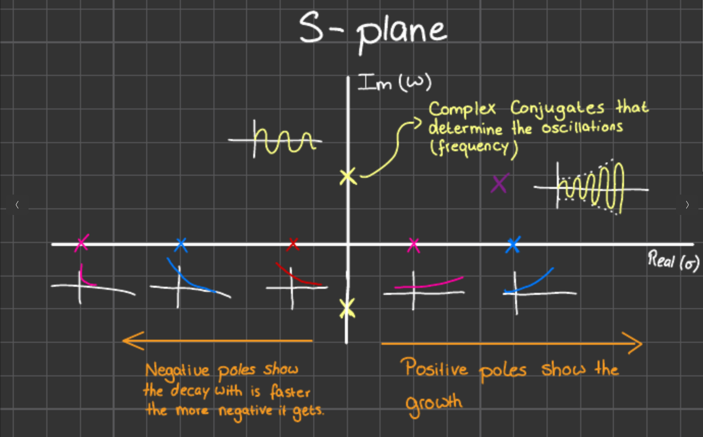
real part of the poles introduces damping…
further away from the origin the faster the decay/gain becomes (real line)
further away from the origin the oscillation frequency increases (imaginary line)
only poles needed to determine stability of the system

Second Order Systems / Fourier Transforms / System Interconnections and Stability

Topic: Fourier Transform

steady state

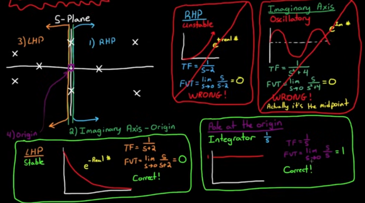
Final Value Theorem → Steady State Gain

Final value exists when it a system converges to a value for example an exponential system diverges and oscillating system without damping does not converge. Meaning only with poles in LHP and Origin

Let ←> be a -transform pair.
If all poles of are in the left-plane, then:

Consequence:
If is a step, , and , then:


is the DC-gain (steady state value of step response) of G

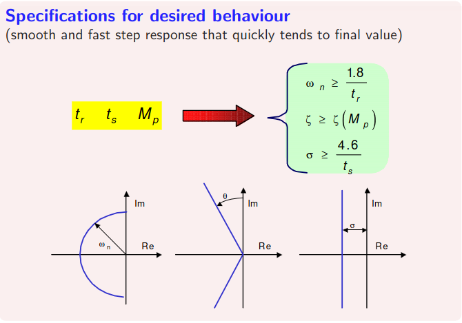
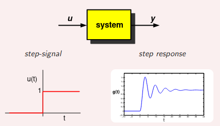
Analytic Express for Step Response:

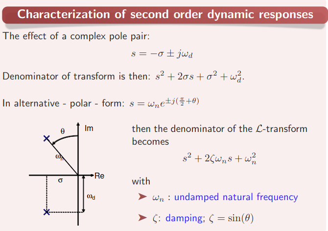
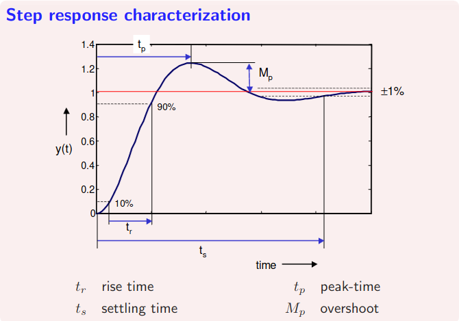
Characterization

Rise time
→
for

Peak time

Overshoot

Settling time

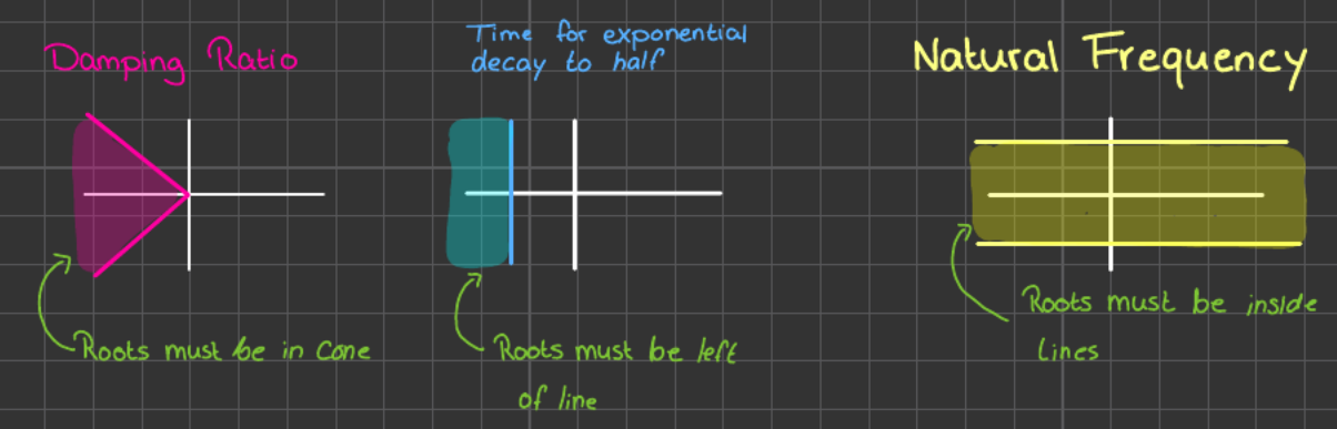
One-to-one relations (2nd order systems)

Consequence of extra zero/pole

Extra Zero
If the effect of the zero is negligible
If not large enough → overshoot increases
If (zero in RHP (right half plane)) initial response can become negative

and if zero in neighborhood of poles (LHP).
Initial negative response if zero in right half plane (RHP)

Extra Pole
if pole is neighborhood of the other poles (LHP)

Stability

An LTI system is called stable if all poles of the transfer function are in the open left half plane, i.e. have negative real parts. (If on imaginery line (critically stable) not stable)

• Routh array → test stability of systems
• Number of sign changes → Number of poles in RHS → Stable: No Sign Changes
• If Routh first column same sign, positive → stable

Routh-stability test of:




Routh–Hurwitz stability criterion - Wikipedia

Bounded input-Bounded output (BIBO) = Stability (absolutely integrable):

Feedback and Feedforward

Topic: Feedback and Stability

• Closed Loop Sensitivity:
• If not a closed-loop system → Routh Stability Check Performed → Before Final Value Theorem
  Types of Systems - YouTube
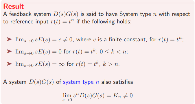
  System Type based on the amount of poles at the origin… Only based for the left hand side poles for stable systems.
  any system of type 2 and higher diverge to infinity for the final value theorem.
  
  

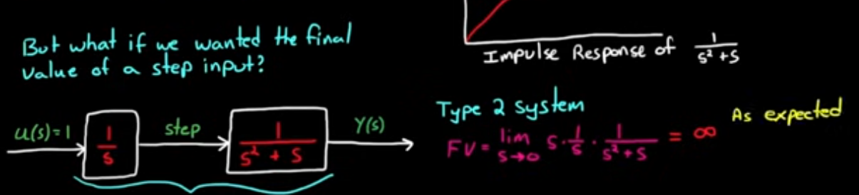
System Types

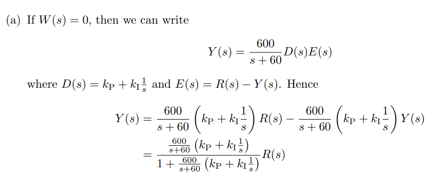
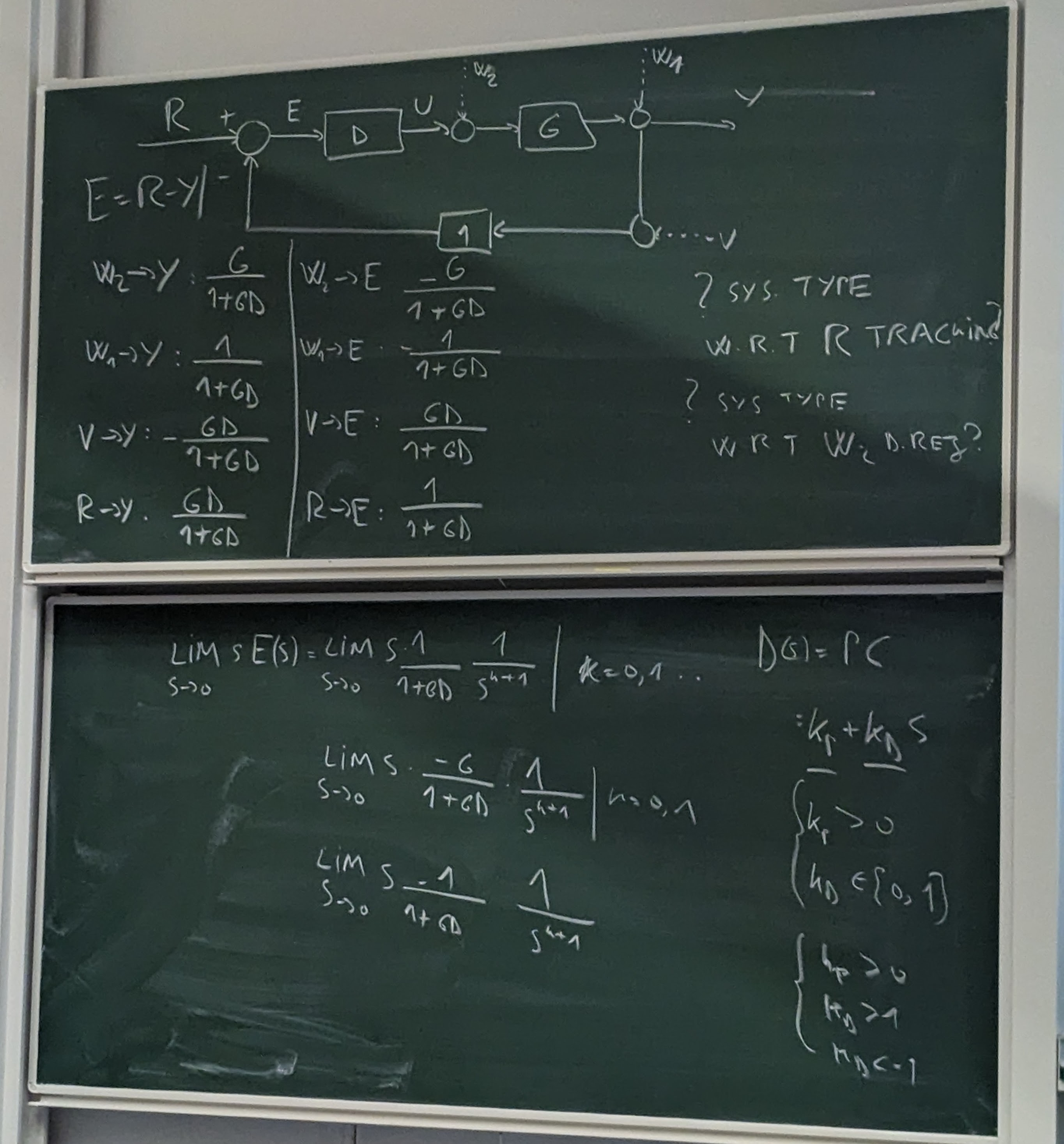
Reference Tracking:

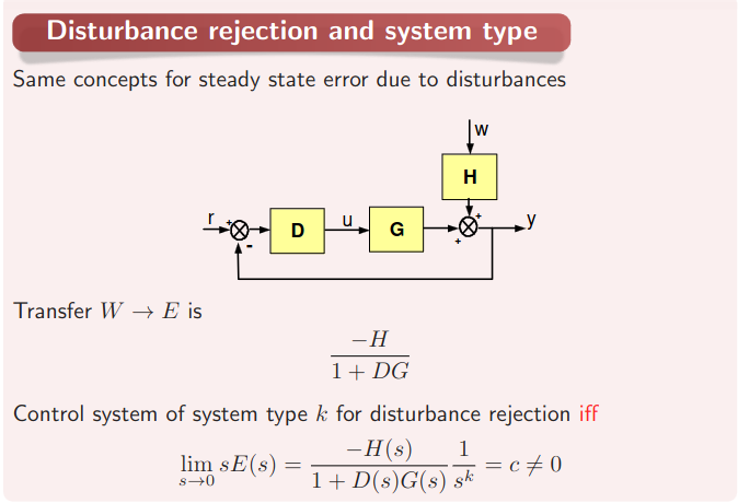
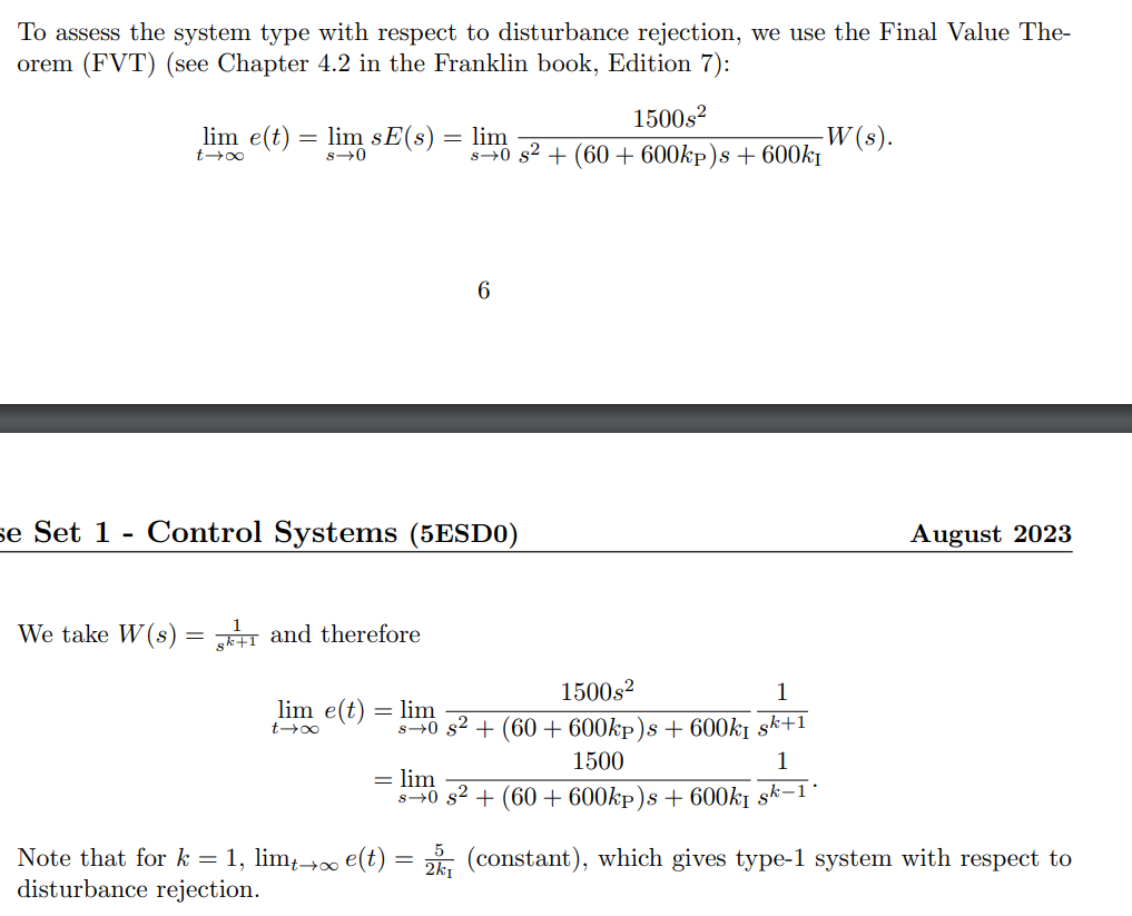
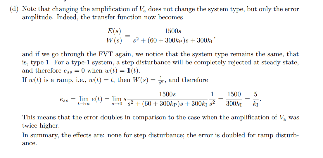
Disturbance Rejection

if that circle H→- then its so numerator
if there is something after that circle lets say Z:

W→E means E=…W

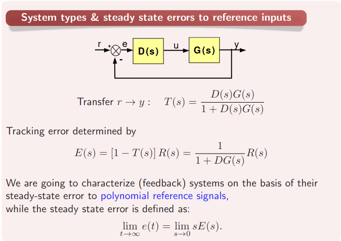
When Reference Tracking - Consider Steady State Errors (R(s))

Final Value Theorem and Steady State Error - YouTube
Role of a closed loop control system is to drive the error(difference between input and output) to zero.




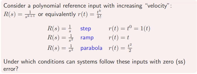
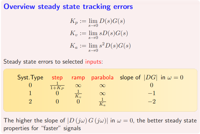
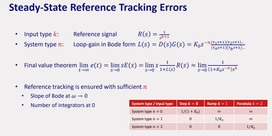
feed forward gain is a way of determining a steady state error when plant and compensator of the system are known.

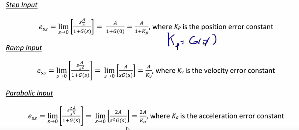
ECE320 Lecture1-3c: Steady-State Error, System Type - YouTube
4.3: Steady-State Error Improvement - Engineering LibreTexts

Feedback Controllers (PID)

Topic: Controller Design
Pid Control Basics In Detail
Simple Examples of PID Control - YouTube
Proportional–integral–derivative controller - Wikipedia

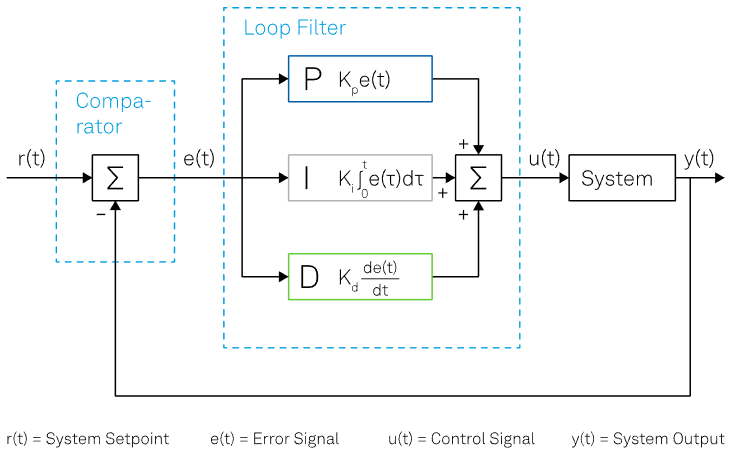
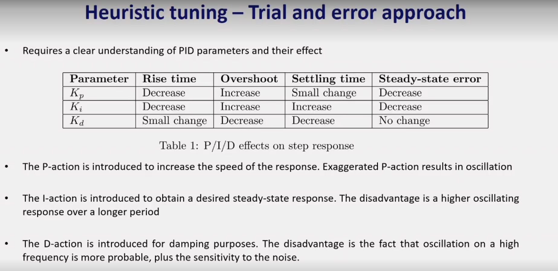
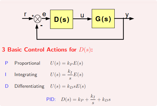
• P used for “speed”
• I used for steady state response
• D used for damping

PID Action in Detail

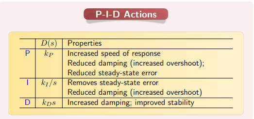
P-action: increase so
faster response less damping

PI-action: leads to zero steady state error to step input.

PD-action: leads to increased damping.