5ESD0 Control Systems
- Area: Signals and Systems
- Topics: Linear Algebra · Laplace Transform · Z-Transform · Sampling · Transfer Functions and Frequency Response · Feedback and Stability · Controller Design · State-Space Models
- Related courses: Systems - 5ESB0 · Signals II (DSP Fundamentals) - 5ESC0 · Math I - 2DE20
Summary
5esd0-summary-samenvatting-control-systems.pdf
Notes
Module 1: Course Introduction (Modifying open-loop transfer function properties using feedback)
Topic: Laplace Transform
Systems - 5ESB0
Module 2: Root Locus (Modifying closed-loop transfer functions using Feedback)
Topic: Feedback and Stability
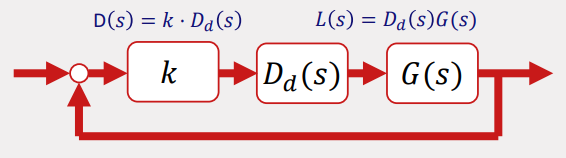
The Root Locus Rules
(VERY USEFUL) How To Sketch a Root Locus
Departure Angle Example
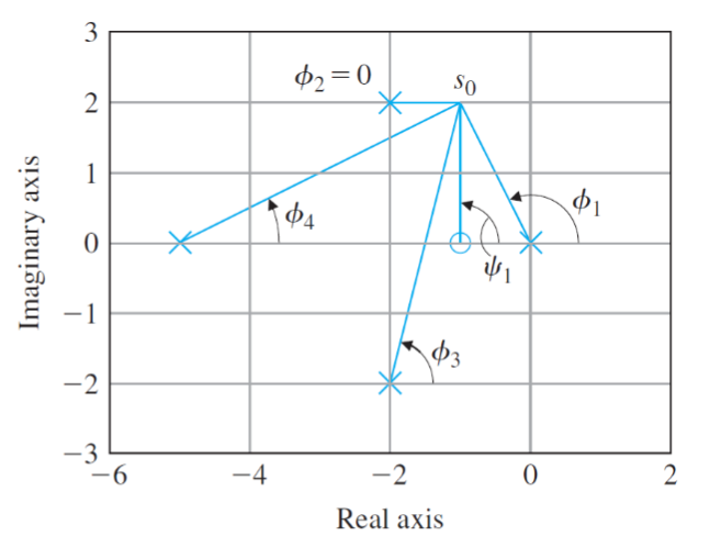
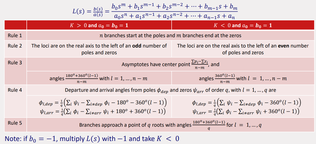
Departure Angles
same just without
Module 3: Frequency Response Functions / Bode Diagrams (Understanding the relevance of frequency-domain control-design methods and frequency-responses on Bode plots)
Topic: Transfer Functions and Frequency Response
Final Exam Tutorial - Bode Plot Example - YouTube
Bode Plots by hand
Bode Plots Explained - YouTube
ChatGPT
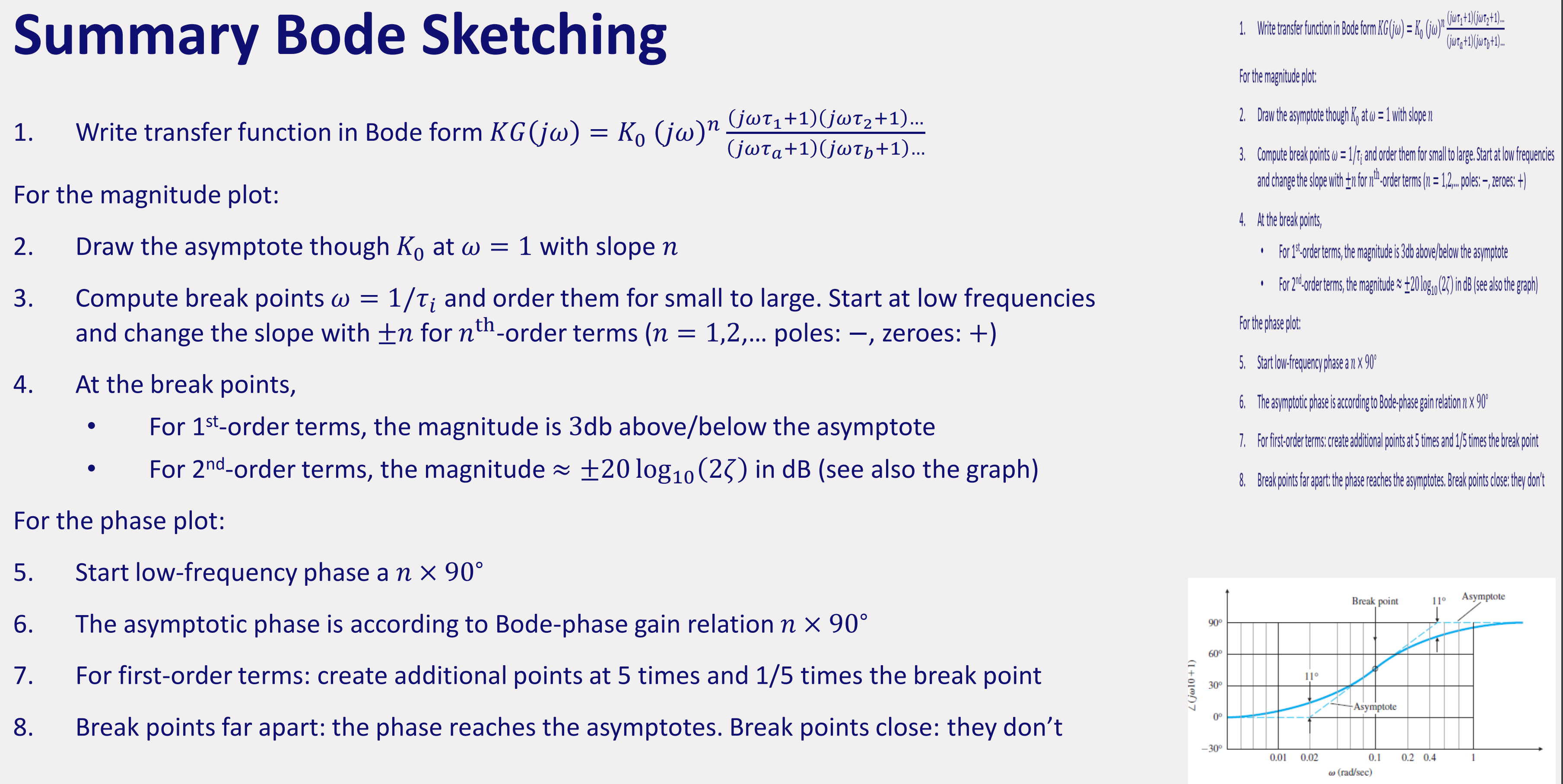
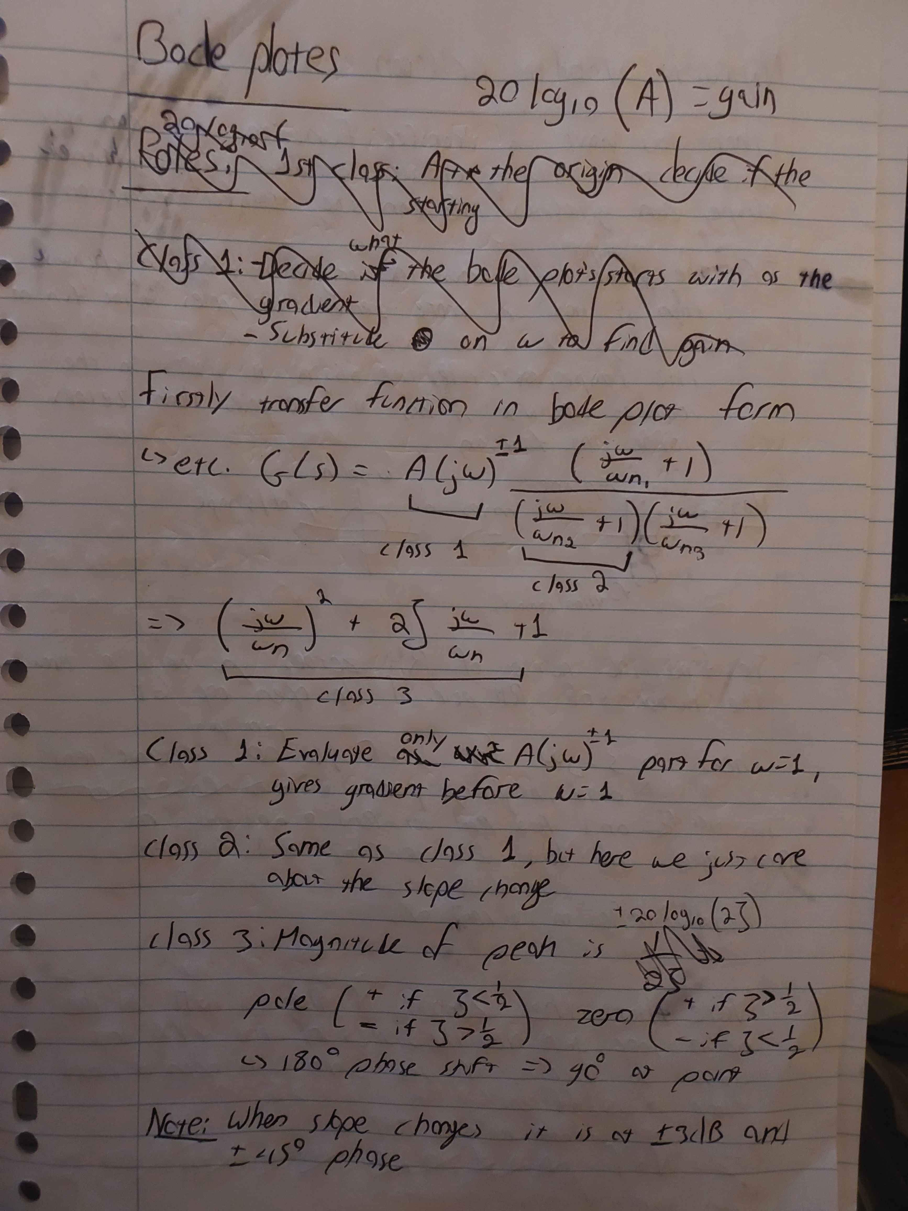
$\text{break point: }\omega=\omega_{n}$
$\text{magnitude asymptote deviations: } \frac{1}{2\zeta}\text{ so }=\pm 20\log(2 \zeta)$
$\text{magnitude slope: }\pm40db$
$\text{phase slope: }\pm180 \degree$
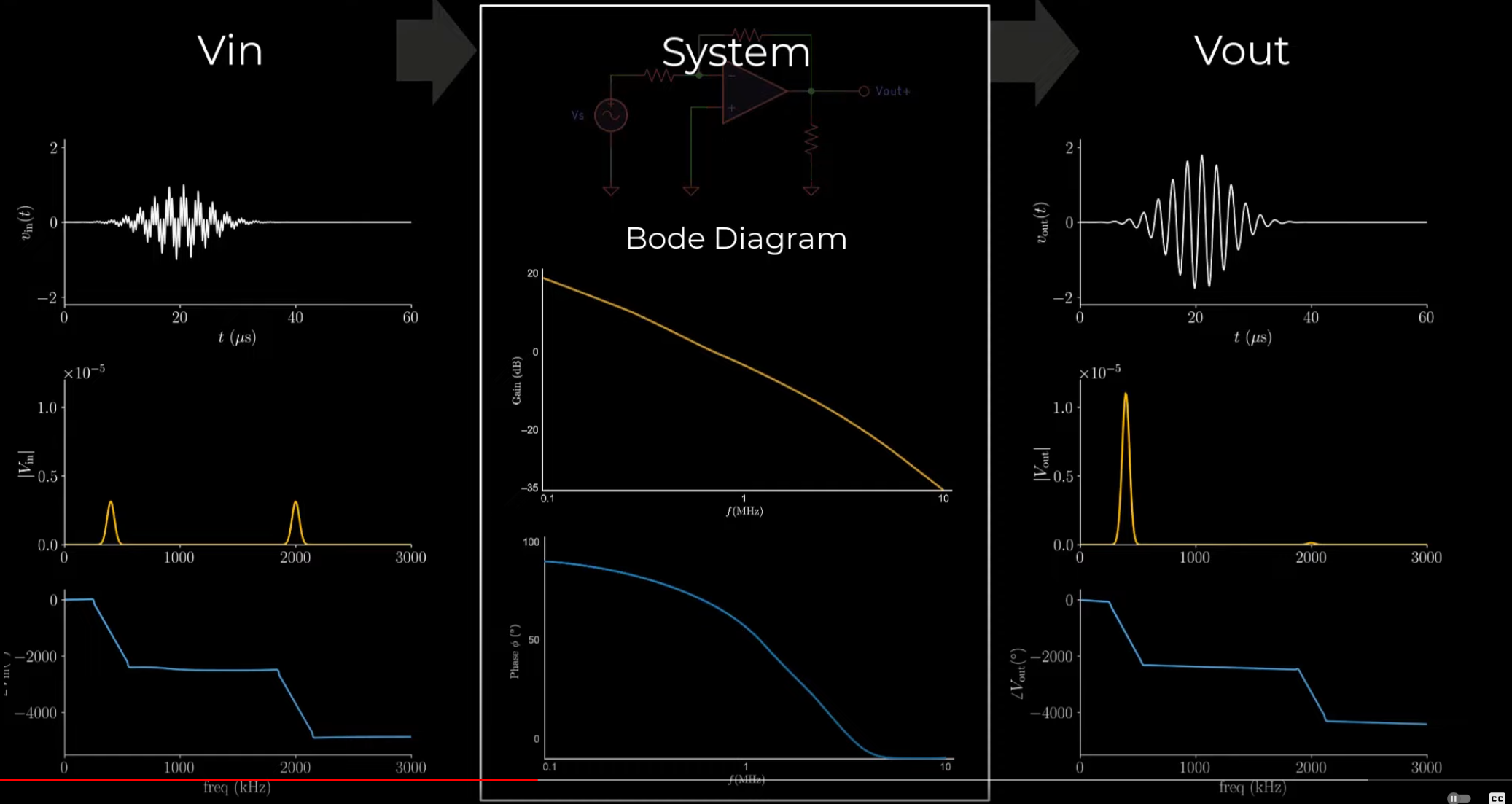
Bode Plots Explained - YouTube
Module 4: Nyquist Stability & Stability Margins (Assessing closed-loop stability and its robustness via Nyquist plots)
Topic: Feedback and Stability
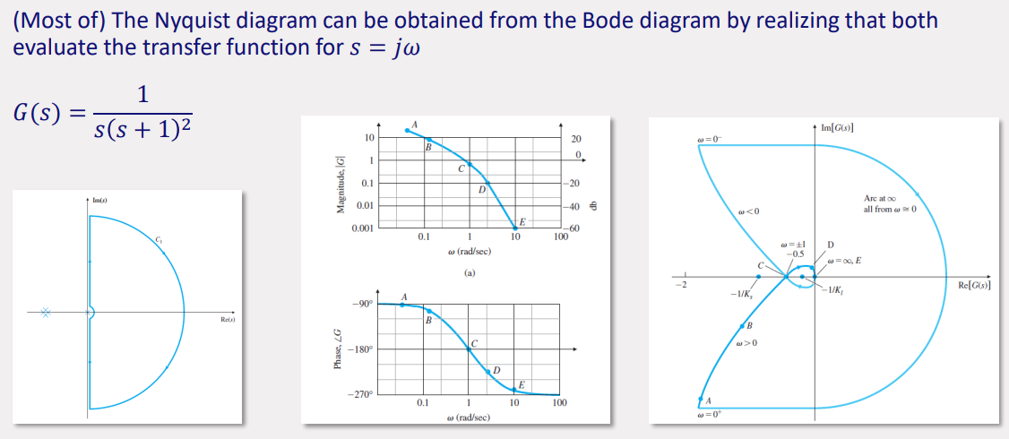
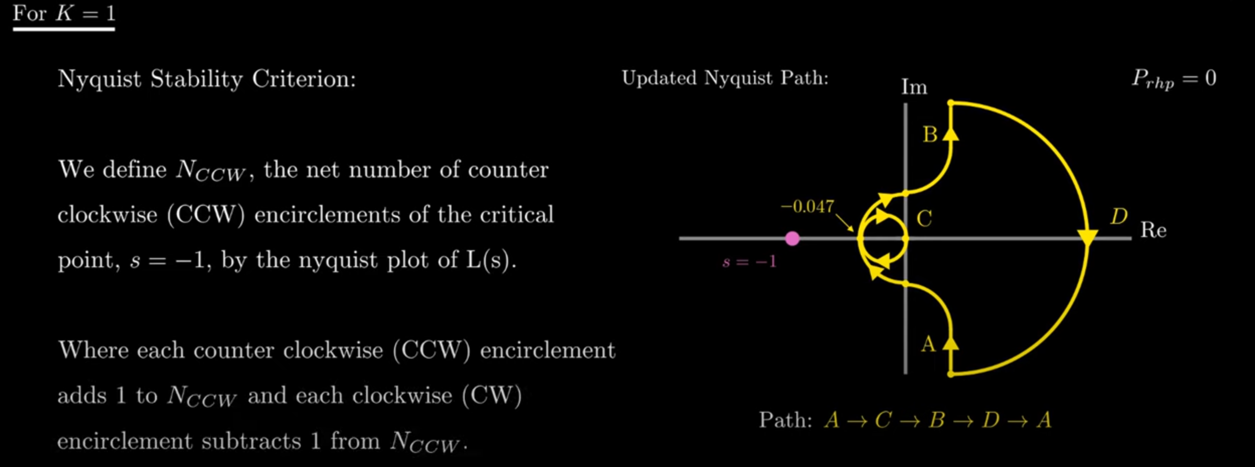
Cauchy’s argument principle
- A clockwise contour map of a complex function will encircle the origin
times, with the number of zeros and is the number of poles of the function inside the contour. - Control Design: 1) Zeros of
are closed-loop poles, 2) contour of interest is one the covers the RHP. - Encirclements of
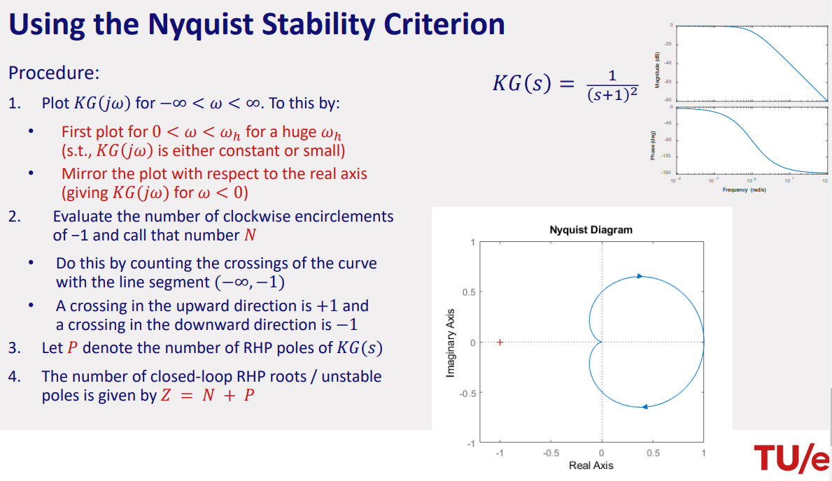
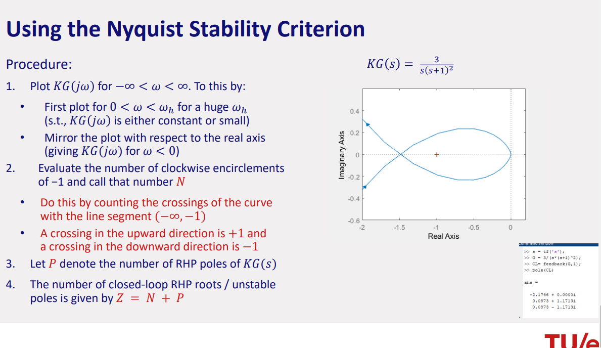
around the origin is equal to encirclements of around -1.
is the number of RHP zeros of (i.e, the closed-loop poles). is the number of (clockwise) encirclements of the point −1. is the number of RHP (unstable) poles of .
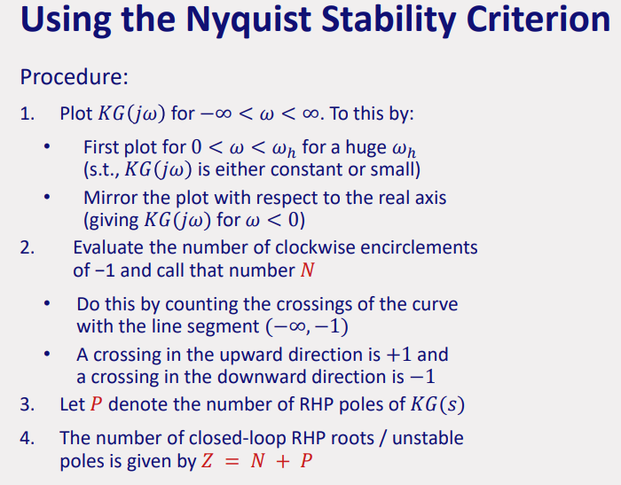
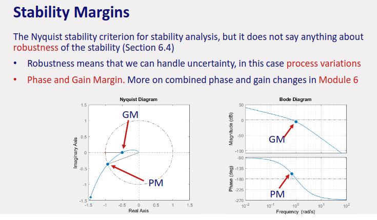
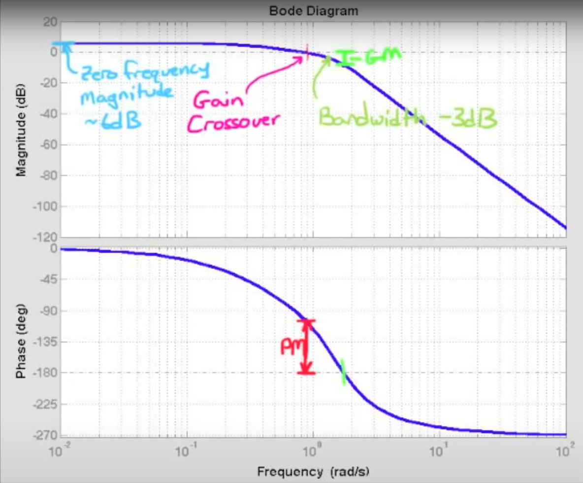
thee amount by which the phase can be decreased before reaching instability.
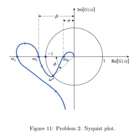
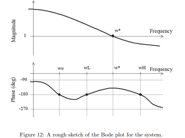
Phase and Gain Margins Example
Final Exam Tutorial - Nyquist Plot Example - YouTube
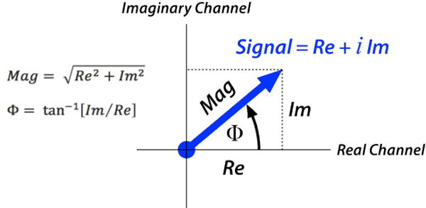
Module 5: Frequency Response Controller Design (Designing single-input-single-output feedback controllers by shaping the open-loop frequency-response function)
Topic: Controller Design
performance specifications
how to tune D for L.
Design feedback controller using open loop response functions.
gain margin is a margin of gain that can be applied to a system since systems IRL can vary a margin is good to have since some have stronger or weaker gain due to mechanical wear-outs.
adding more than needed amount of integrator poles effects the phase margin and puts more requirements on the lead/lag compensator.
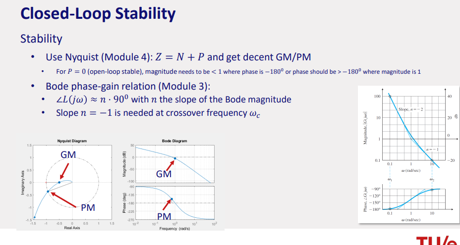
stability margins
Nyquist plot, having a certain PM and GM
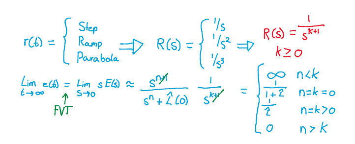
steady state error tracking
controlled by system type.
steady state error → 0 if slope of the bode diagram of L(s) is steep.
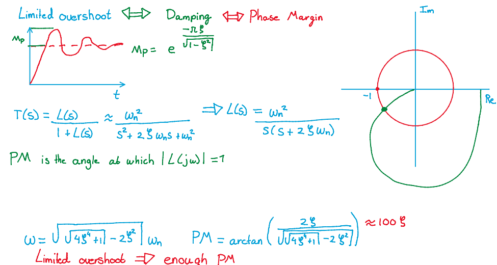
overshoot
enough phase margin
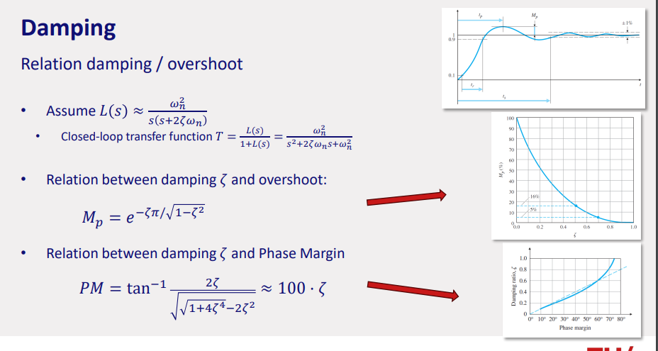
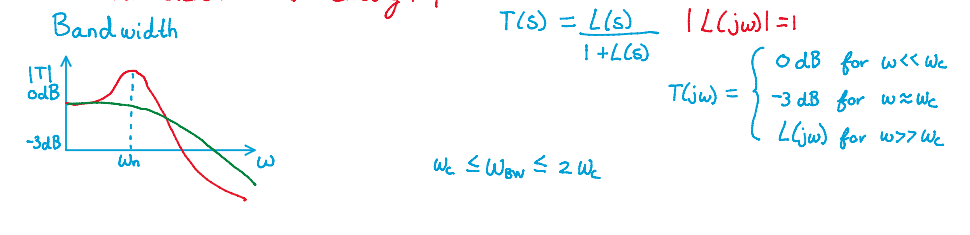
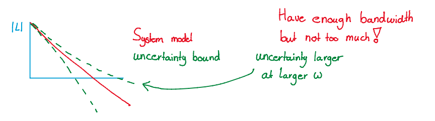
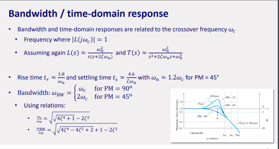
closed loop bandwidth
crossover frequency
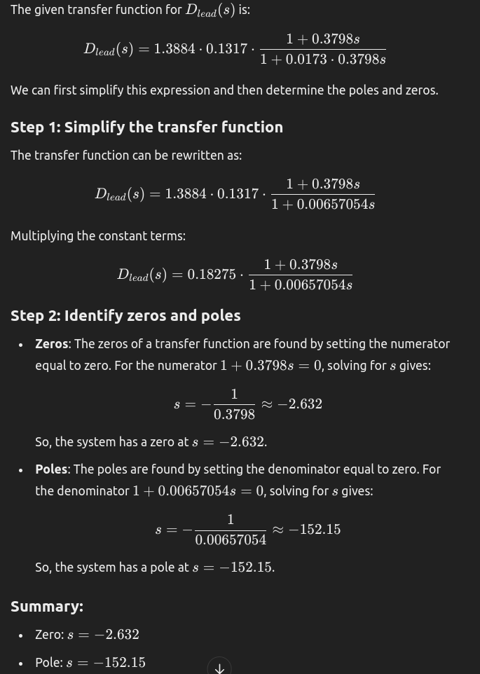
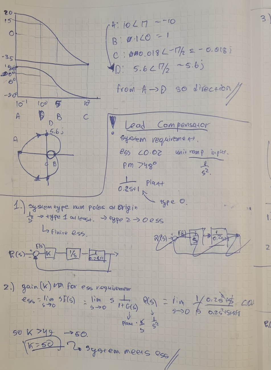
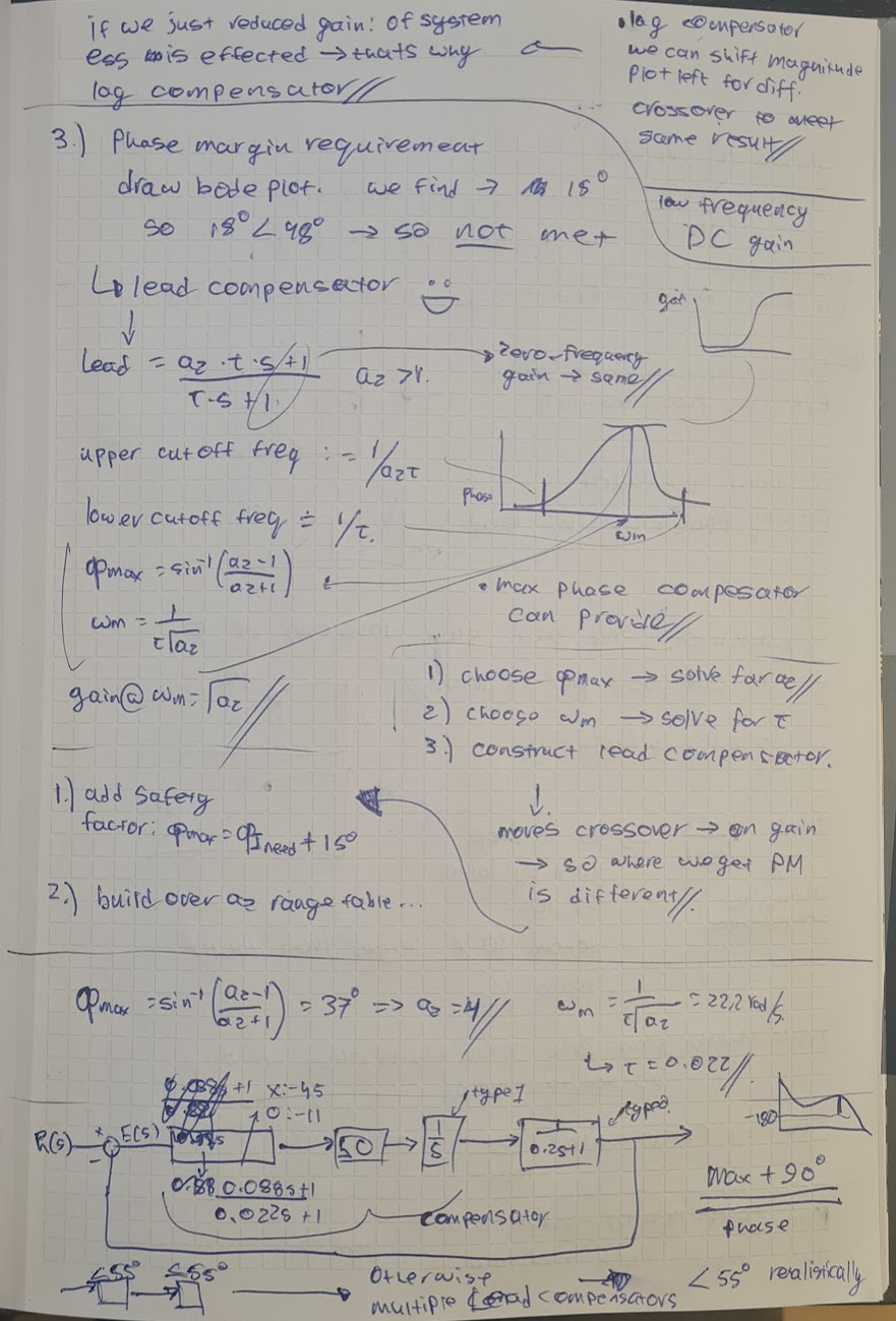
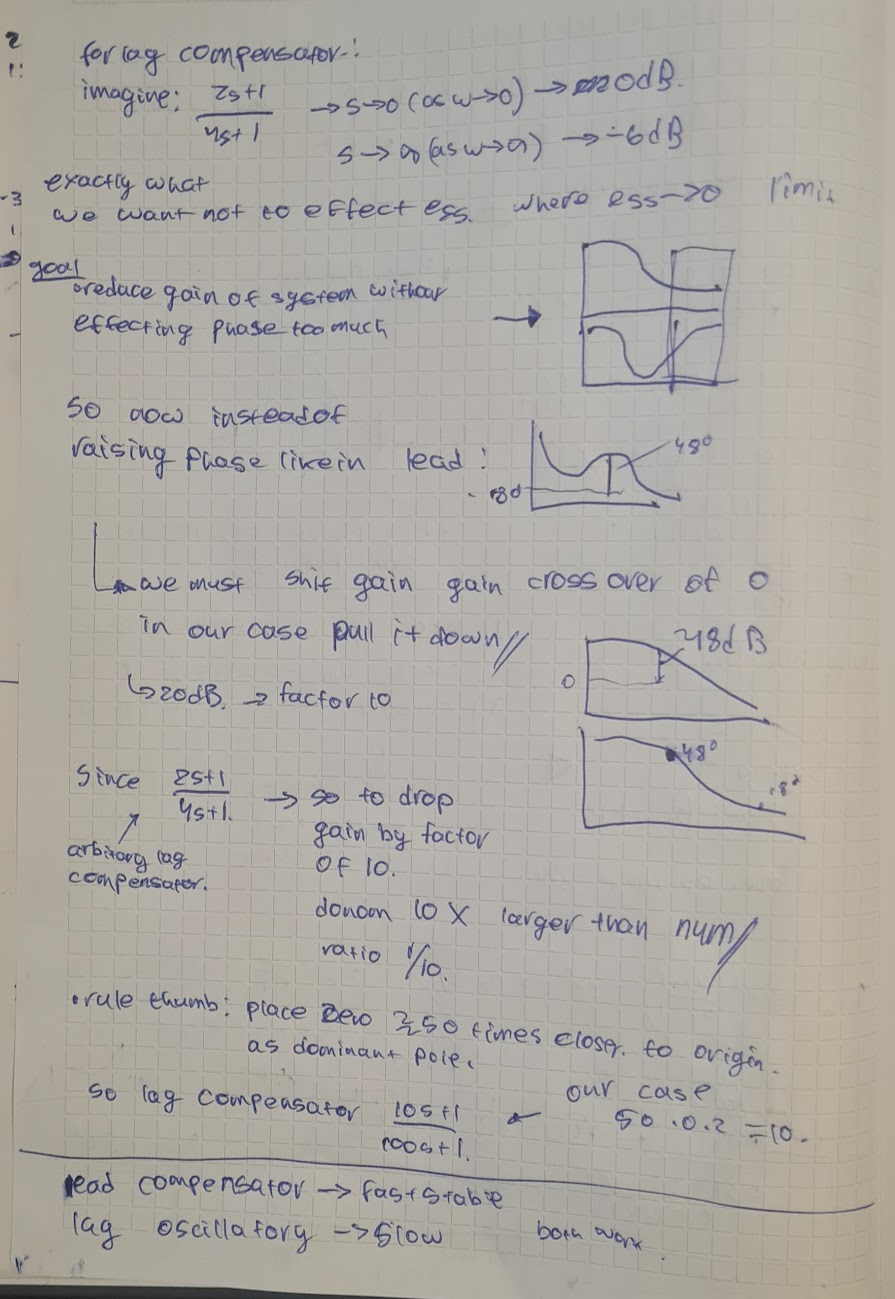
compensators
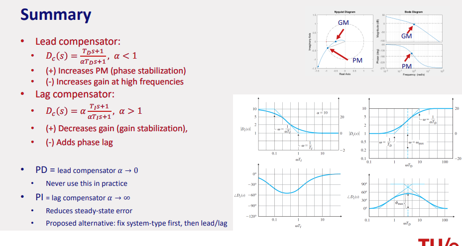
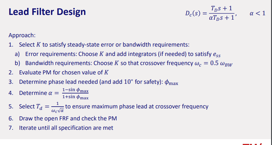
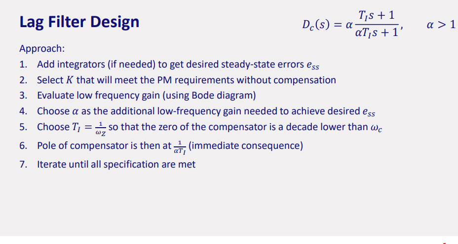
lead lag intuitive understanding
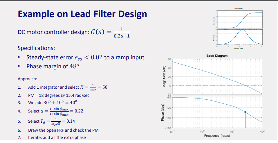
lead: adds phase lead to the system increasing gain (between zero → pole)
(typical goal to provide gain in high frequency range).
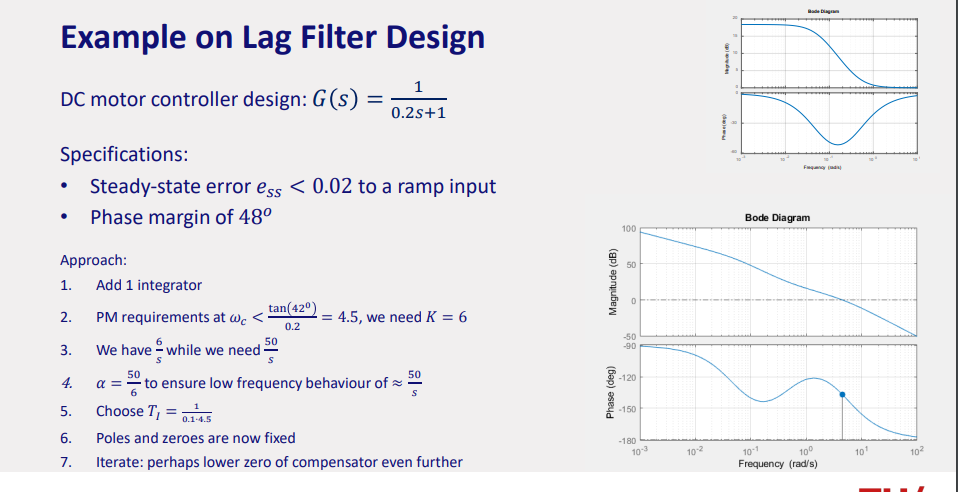
lag: adds phase lag to the system decreasing gain (between pole → zero)
(typical goal to provide gain in low frequency range).
(max
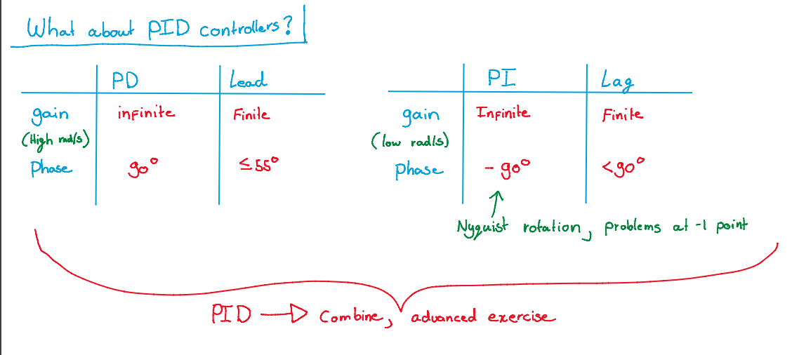
lead lag compensators
zeros add
poles subtract
example of lead (opposite for lag), cancels if pole zero at same:
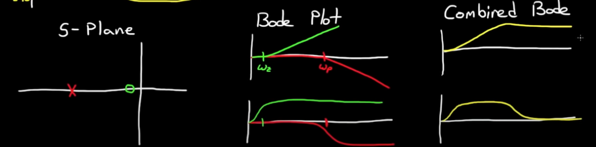
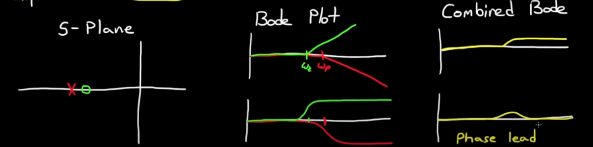
lead/lag: to amplify at lower and attenuate at higher…
Designing a Lead Compensator with Bode Plot - YouTube
Designing a Lag Compensator with Bode Plot - YouTube
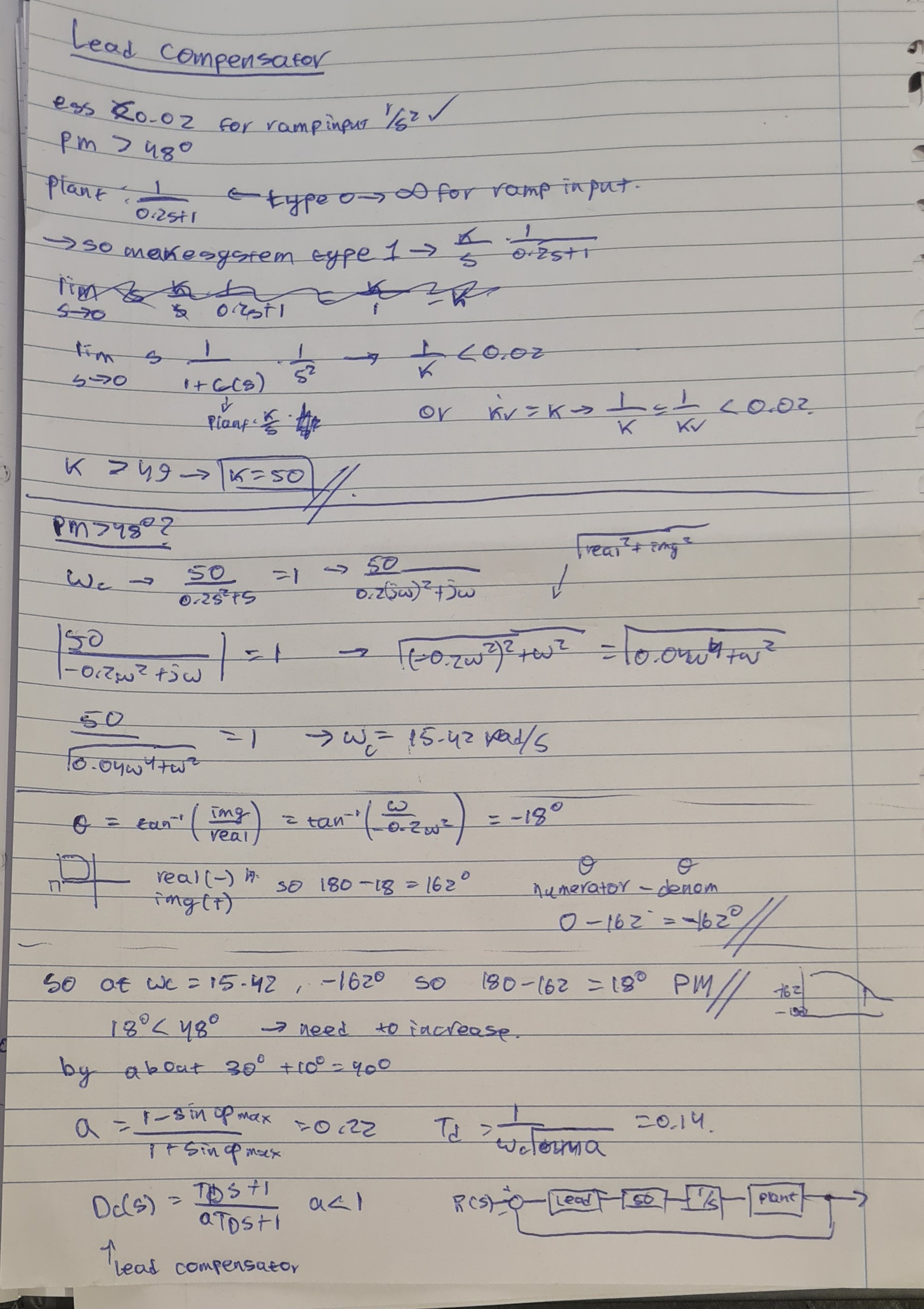
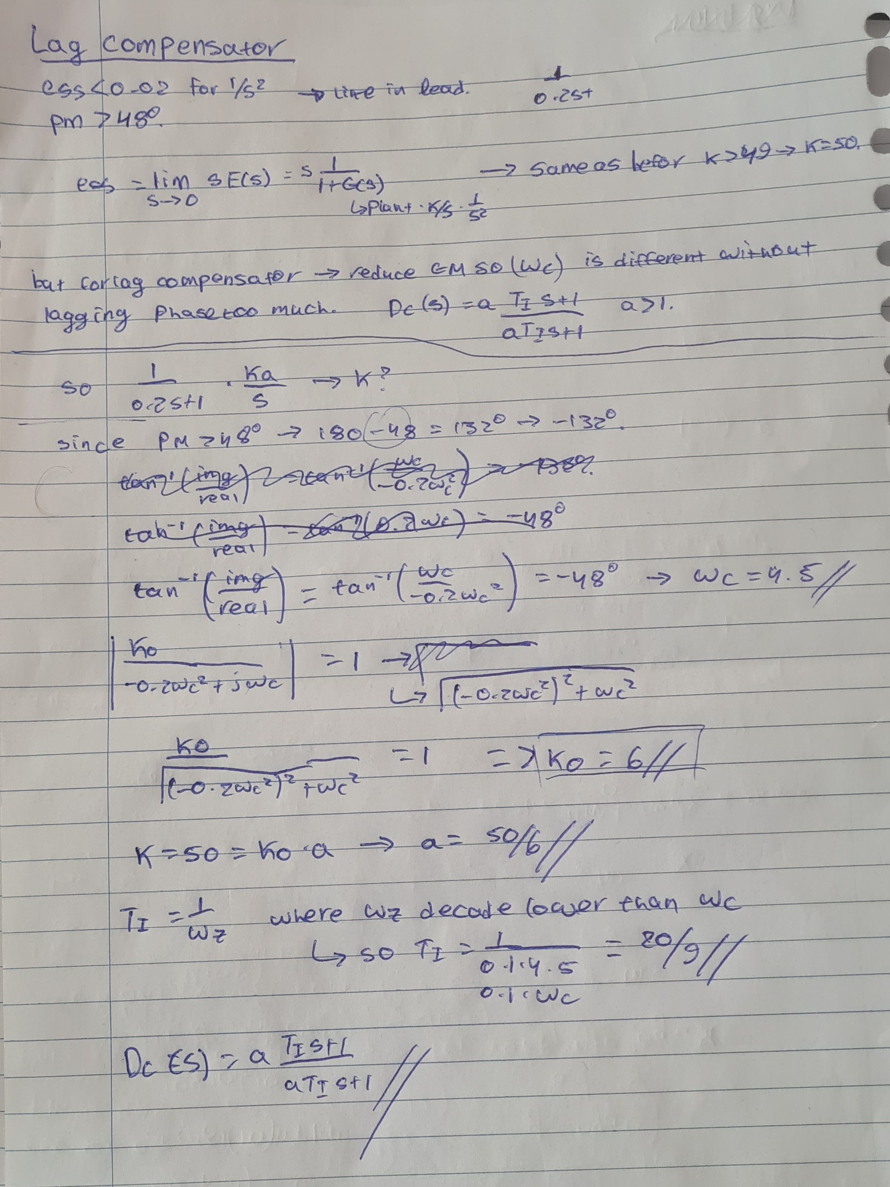
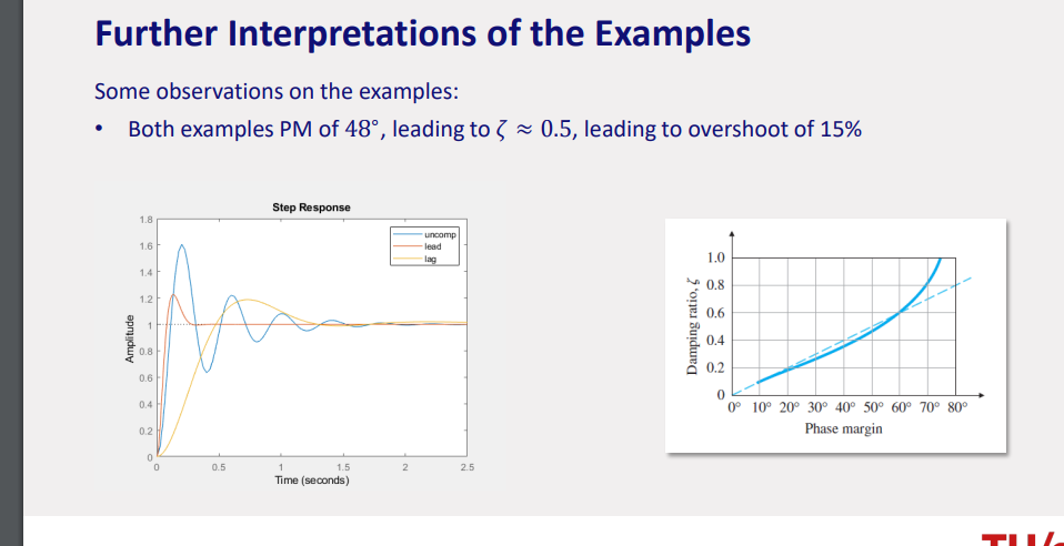
usually lead filter have higher cross over frequency…
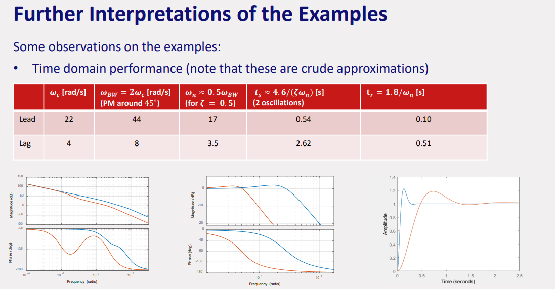
other compensator pics
Module 6: Fundamental Limitations in Control Design (Identifying the limitations of linear control design, and the trade-off between disturbance rejection and sensor noise amplification)
Topic: Controller Design
General knowledge
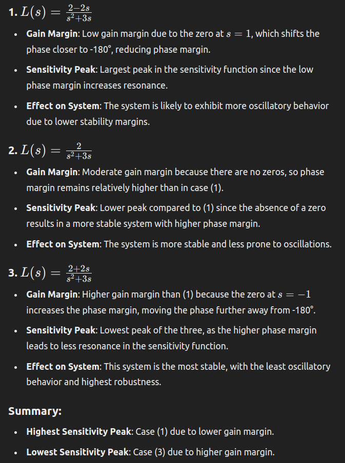
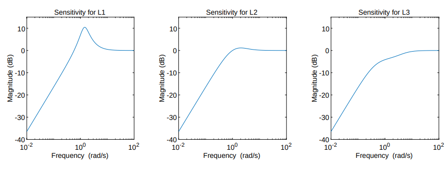
By analyzing the sensitivity function in the logarithmic bode scale we have derive robustness and performance limitations.
If I want to reduce sensitivity with regards to tracking references, then I can make system susceptible to measurement noise.
Peak of sensitivity and how it relates to nyquist
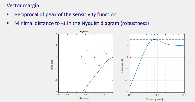
The peak of the sensitivity function represents how much the system amplifies disturbances. It is the reciprocal of the smallest distance from the Nyquist plot to the critical point
Bode sensitivity integral
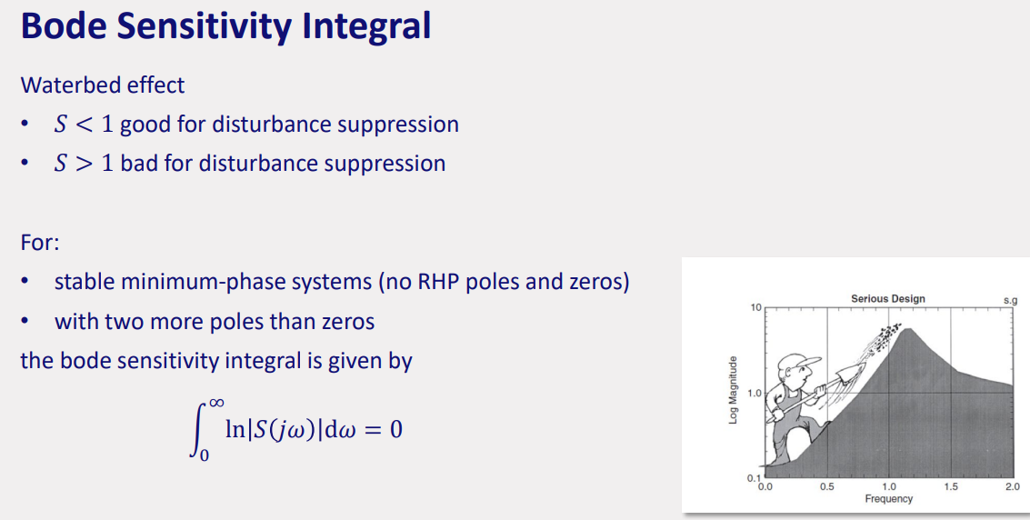
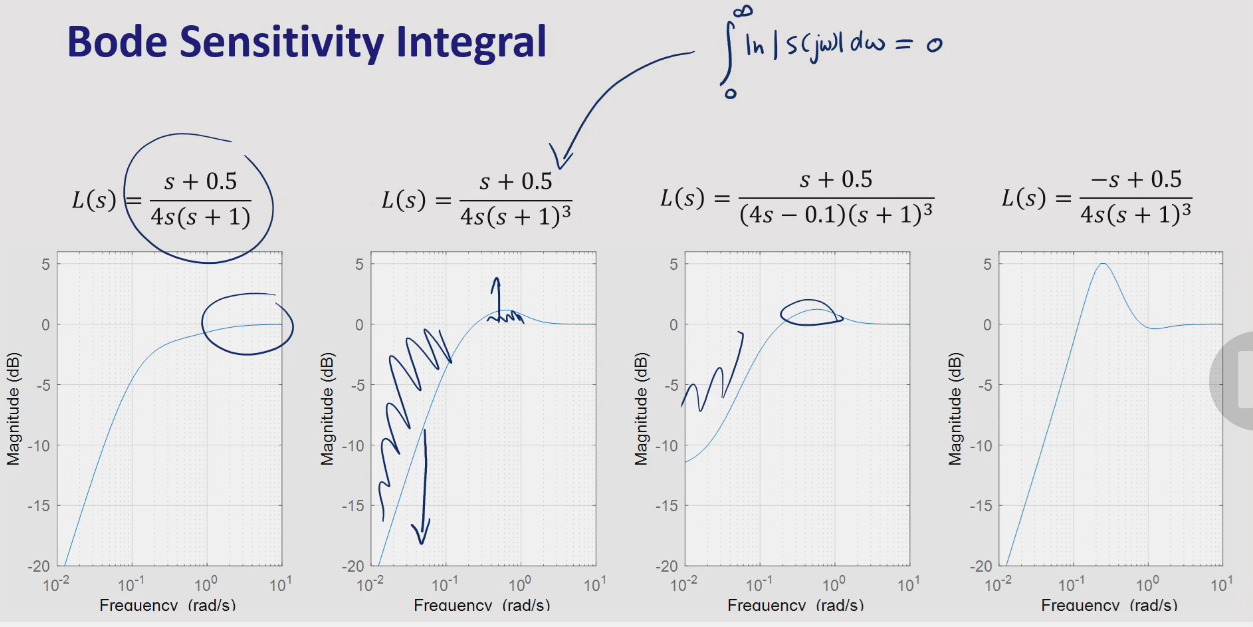
improving characteristics in one range make them worse in the other range…
Cauchy’s integral:
numeric effects when placing poles or zeros in specific spots based on waterbed effect…
Control system types
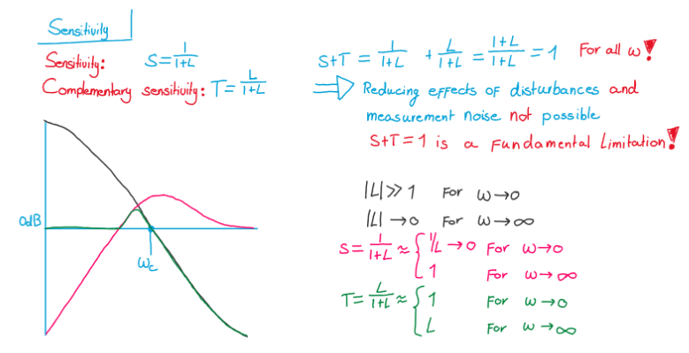
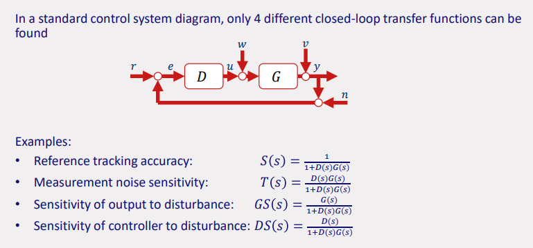
sensitivity is looked at when asked about maximal disturbance
complemetary sensitivity is looked at when asked about maximal disturbance
overall:
fight disturbances
fight measurement noise
Performance Limitations of Right Half Plane (RHP) Zeros
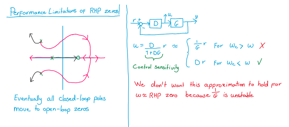
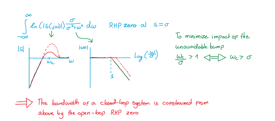
- Explanation: When there are RHP zeros, closed-loop poles eventually approach these zeros as the loop gain increases. This causes limitations in control performance, especially at higher frequencies.
- Math:
Performance Limitations of Right Half Plane (RHP) Poles
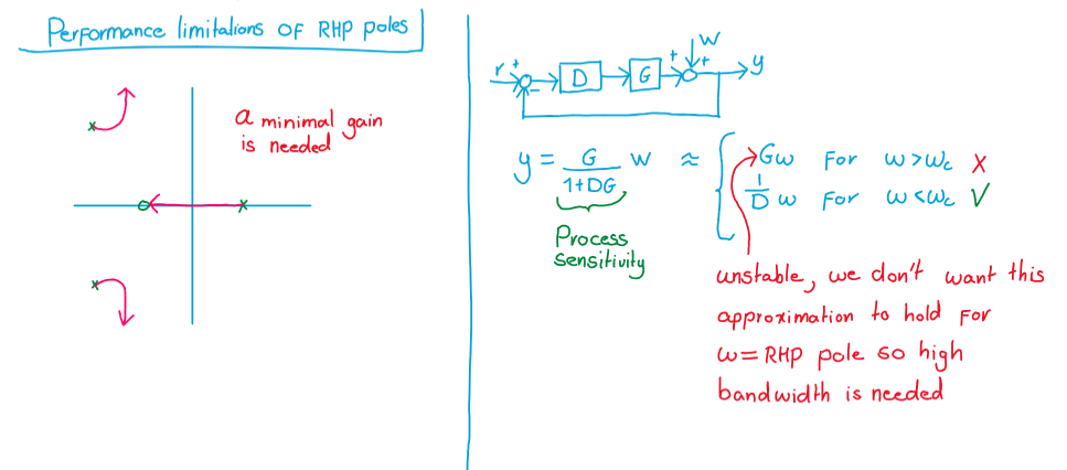
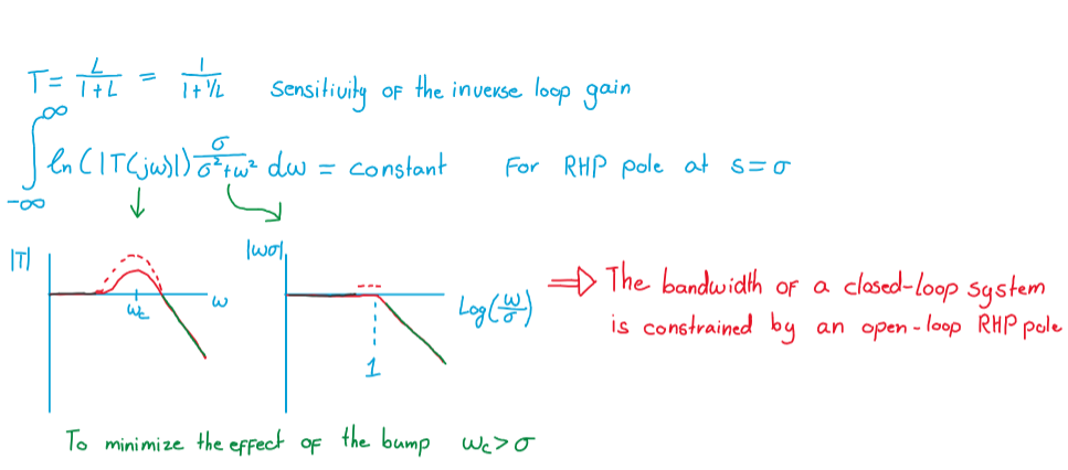
- Explanation: RHP poles require a minimal gain for stability. As frequency approaches the RHP pole, the system needs higher bandwidth to maintain stability.
- Math:
exercise
Module 7: State-Space Models (Understanding the relevance of state-space control design, and the analysis of the state-space equations)
Topic: State-Space Models
State-space representation - Wikipedia
Math I - 2DE20
transpose, product, inverse, rank, eigenvalues, eigenvectors
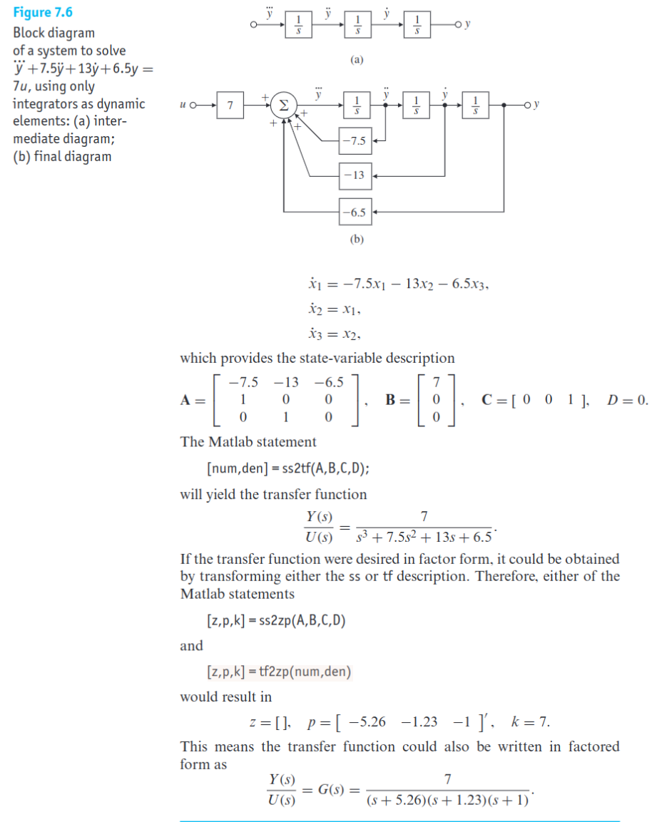
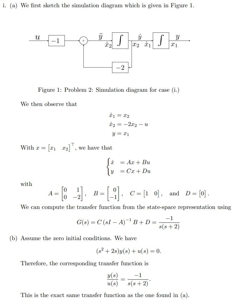
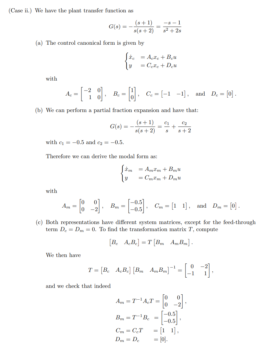
deriving state space models
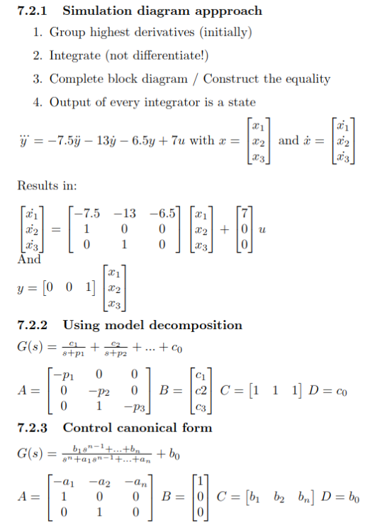
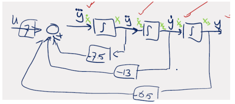
Simulation Diagram, Modal Decomposition, Control Canonical Form.
block diagram to state space - YouTube
state space analysis
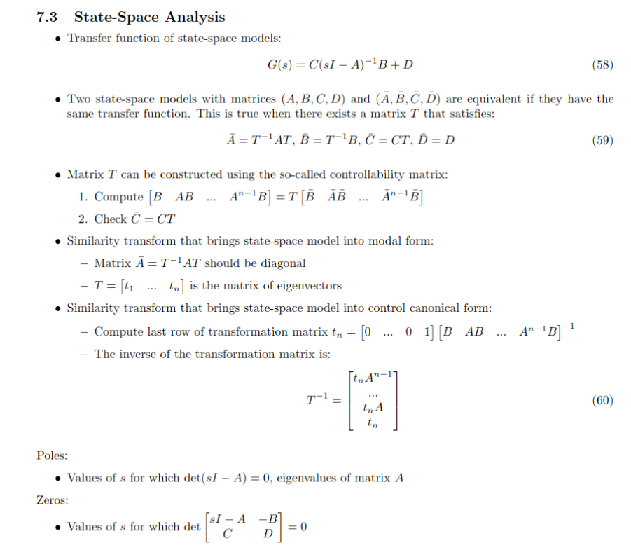
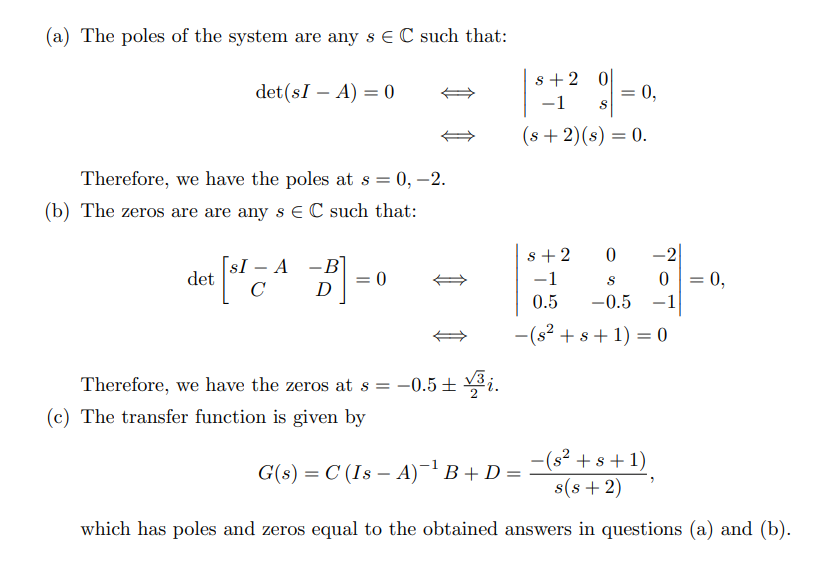
TF from SS:
- poles of the transfer function are the eigenvalues of the system matrix
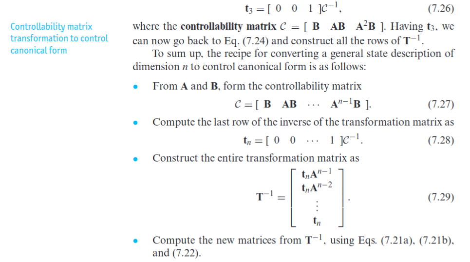
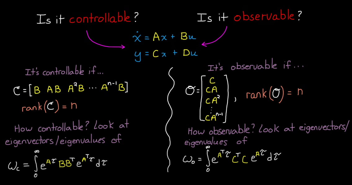
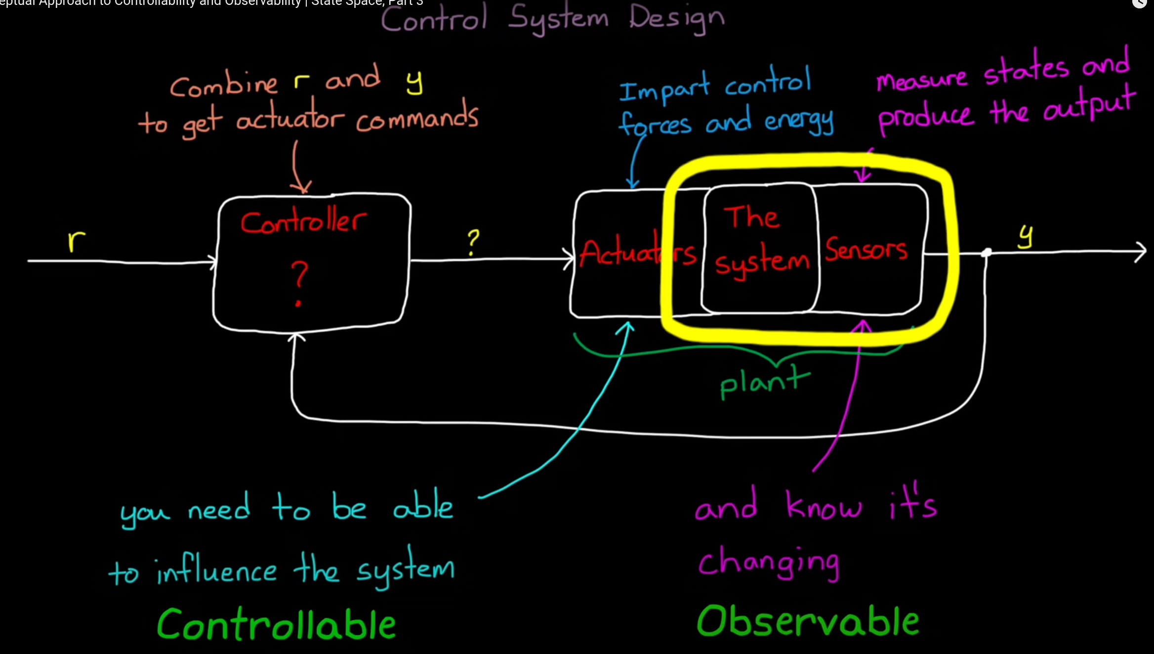
controllability: reach a specific state (not maintain)
observability: core states in A matrix
if you look above
we mainly work with control canonical form but there is also observer canonical form
linearisation of SS models
- Write
- Use taylor series to obtain:
extra
Module 8: State-Space Control Design (Designing state-space controllers via the pole-placement)
Topic: State-Space Models
pole placement is a fancy root locus with placement across matrix not just locus lines…
8.1 Recap Eigenvalues / Eigenvectors / Determinants
Topic: Linear Algebra
- Eigenvector condition: For
, vector is an eigenvector if it satisfies . - Eigenvalue computation:
(non-trivial ) → solve . - Key points:
- Eigenvalue
: scalar associated with eigenvector . - Eigenvector
is in the nullspace of .
- Eigenvalue
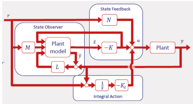
8.2 State-Space Control Design
- Plant model:
, - State Feedback:
- State Observer:
- Integral Action (when
):
8.3 Controllability / Observability
- Controllability: Ability to control each state (actuator/sensor location).
- Controllability Matrix
:
- Observability Matrix
:
- Conditions:
- Controllable if
- Observable if
- Controllable if
8.4 State Feedback
Topic: Controller Design
- Controller Design:
to achieve . - Design of Matrix
: - Transform plant to control canonical form.
- Use desired characteristic polynomial
. - Compute
, or use MATLAB placecommand.
- Matrix
for steady-state reference tracking:
where
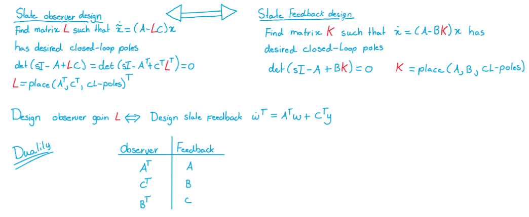
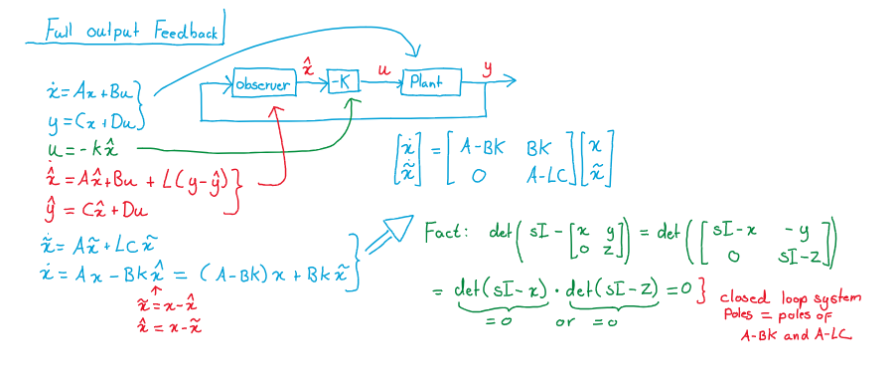
8.5 Observer Design
-
Controller Equations:
-
Observation Error:
-
Matrix
: Controls transient response of observation error. - Duality of control and estimation: closed-loop poles of
- Separation Property: Stable state feedback + stable estimation error = stable closed-loop.
- Duality of control and estimation: closed-loop poles of
-
Matrix
for tracking: - If
, estimation error is independent of reference. - Set
and for “classical control scheme”.
- If
8.6 Reference Tracking
- State Feedback:
- No feedback path with
; no integral action.
- No feedback path with
- Inexact Plant Model Tracking:
- Augment plant with integrator:
- Augment plant with integrator:
- Controller Structures:
- Case 1:
and : - Case 2:
and : - Case 3:
, , add integral action:
- Case 1:
Module 9: Digital Control (Addressing the limitations of controller design due to sampling, and the limitation of experimental platforms)
Discrete control #5: The bilinear transform - YouTube
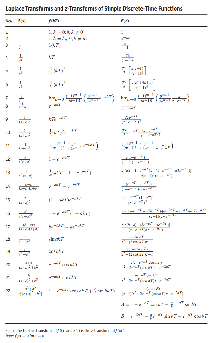
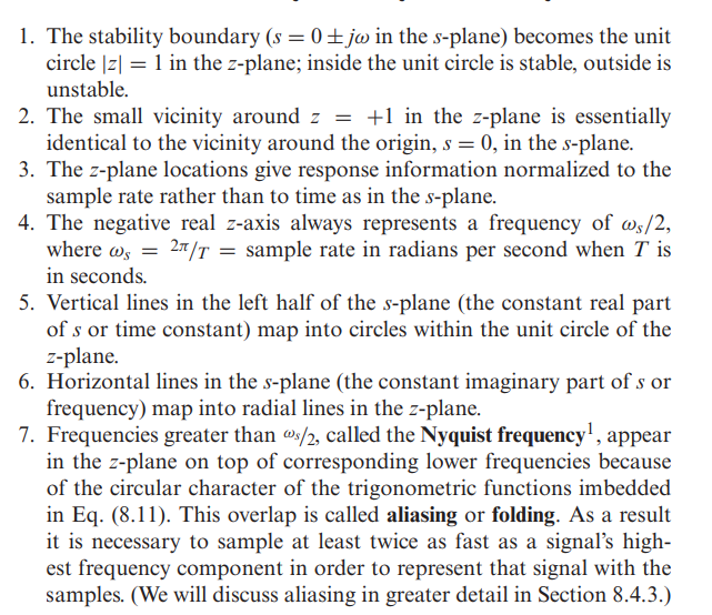
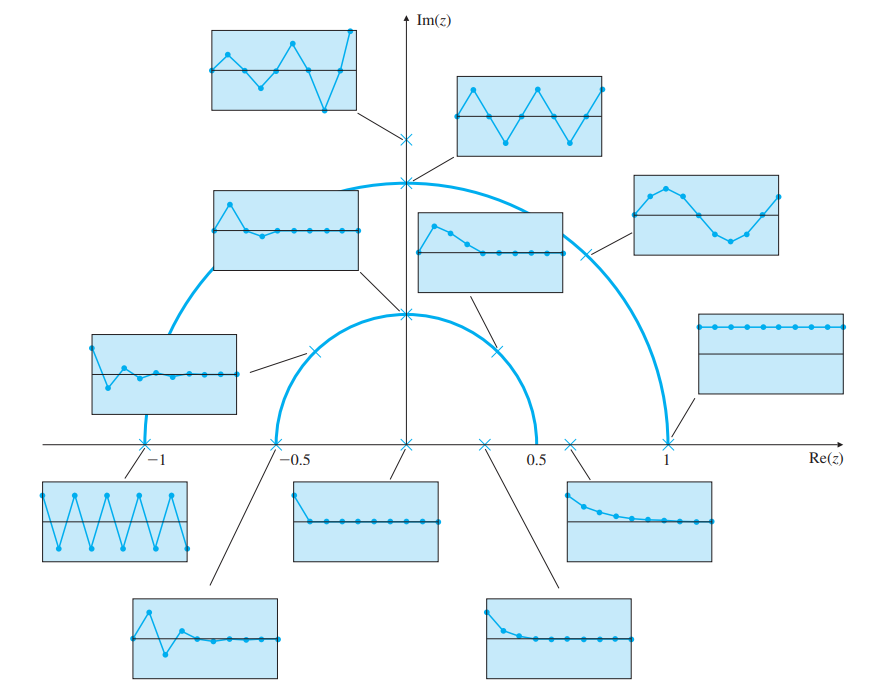
The s-domain’s left half-plane maps to the area inside the z-domain’s unit circle, while the s-domain’s right half-plane maps to the area outside of the z-domain’s unit circle.
9.1 Artifacts Introduced in Digital Control
Topic: Sampling
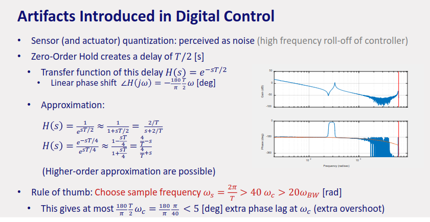
- Sensor quantization: perceived as noise.
- Zero-Order Hold (ZOH) creates a delay of
. - Transfer function of this delay:
- Linear phase shift:
- Approximation:
- Rule of thumb: Choose sample frequency
- Transfer function of this delay:
9.2 The Z-domain
Topic: Z-Transform
- Stability: Unit circle instead of Left-Hand Plane.
- Mapping:
represents a forward time shift, is a derivative in Laplace.
9.3 Three Different Mappings
Topic: Z-Transform
- Matched pole-zero:
(rarely used). - ZOH: Used for discretizing plant to create discrete-time controller.
- Solve
. - Compute
, then do partial fraction expansion.
- Solve
- Tustin: Used for discretizing controller.
- Replace
- Lead/lag filter:
- Replace
9.4 Two Different Design Approaches
- Design CT controller, then discretize:
- Take sampling delay into account (increases phase margin, PM).
- Use
. - Discretize controller using Tustin/Bilinear transform.
- Discretize CT plant to DT, then design DT controller:
- Example:
, let and .
- Sampling delay is considered; DT is not stable for all
because of sampling (in CT: RHP zero). - Design controllers using standard techniques (Root locus, Nyquist, loop shaping).
- Example:
9.5 Compensation in Discrete-Time
- Proportional compensation:
- CT:
- DT:
- Apply ZOH rules.
- CT:
- Derivative compensation:
- CT:
- DT:
- Apply ZOH rules.
- CT:
- Integral compensation:
- CT:
- DT:
- Apply ZOH rules.
- CT:
- Lead/lag compensation:
- CT:
- DT:
- The relation between
is not straightforward but not critical for design.
- CT: