Components in Wireless Technologies - 5XTC0

5XTC0 Components in Wireless Technologies

• Area: Electromagnetics and Waves
• Topics: Noise · Transmission Lines · Antennas and Radiation · S-Parameters and Impedance Matching · Wireless Channel
• Related courses: Electromagnetics II - 5EPB0 · Communication 1 - 5ETC0 · Bachelor End Project - BEP

Schedule

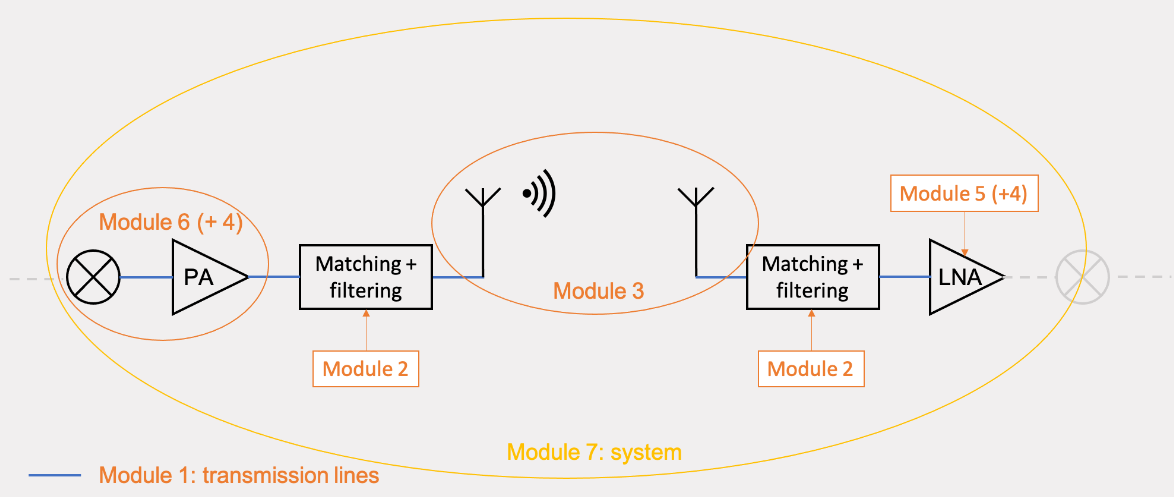
Overview

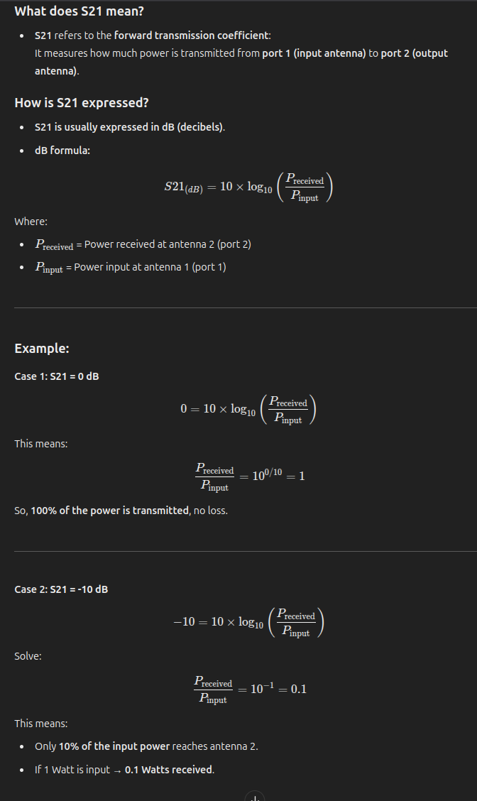
S-Parameters for Antennas (S11, S12, …)

Transmission Lines

Topic: Transmission Lines

5XTC0_Lecture_Module1_TL-Theory_2025.pdf

Formulas

Telegrapher Equations (Time Domain):

Telegrapher Equations (Frequency Domain):

Wave Equations (Voltage and Current):


where

General Solution (Wave Propagation):

Characteristic Impedance:

For lossless lines:

Lossless Line Parameters:

Reflection Coefficient at Load:

Voltage and Current on Terminated Line:

Input Impedance at Distance from Load:

Quarter-Wave Transformer Matching Condition:

if line length

Transmission Coefficient:

Insertion Loss (dB):

Smith Chart Reflection Phase Relation:

other

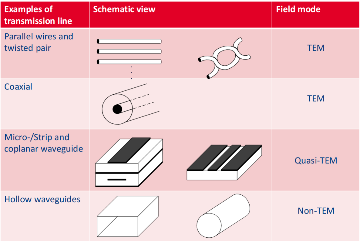
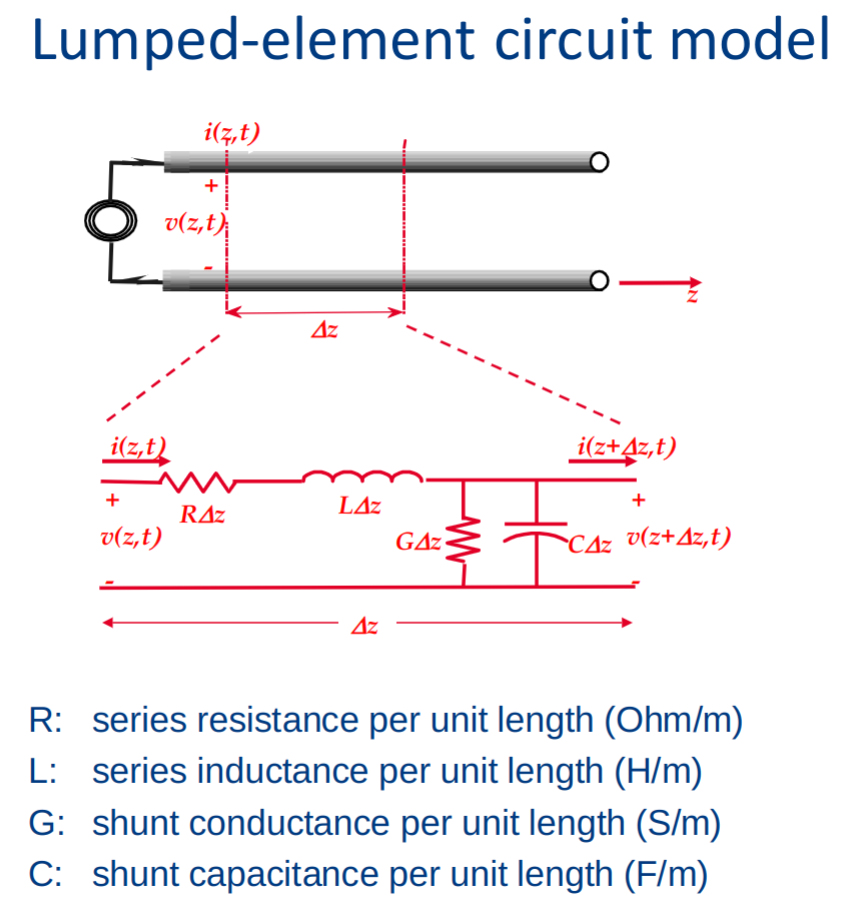
Telegrapher equations

KVL and KCL:

Time domain:

Frequency domain:

Wave propagation on a transmission line

and
solving the above further the telegraph equations produce:
and
complex propagation constant: where is attenuation and is phase constant.

Wave propagation on Tline

The voltage and current along a transmission line can be expressed as the sum of forward and backward traveling waves:

Derivation of the Voltage Equation

The spatial derivative of voltage along the transmission line is given by:

Using the Telegrapher’s equations, this is also equal to:

Substituting :

Expressing Current Components in Terms of Voltage

From the above equation, we can solve for and :

Characteristic Impedance of the Transmission Line

The ratio of voltage to current defines the characteristic impedance:

is the characteristic impedance of the transmission line, which determines how waves propagate and reflect along the line.

The lossless transmission line

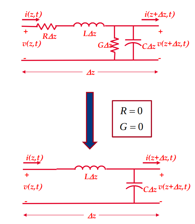
Total voltage and current:

Total voltage and current at the load at :

Special cases:

short circuit load: open ended load: matched load:

Rewriting:
reflection coefficient

Terminated Transmission Line Equations

connected a resistance at the end of transmission line, so pulse sees same impedance at the end as it did propagating.

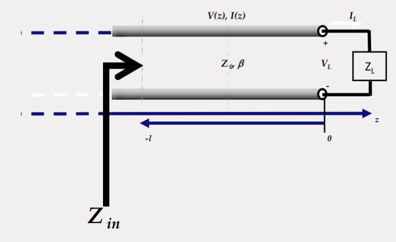
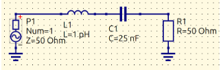
LC lumped element (resonator) as load:

Insertion Loss

Insertion loss quantifies the power loss when two transmission lines with different characteristic impedances are connected.

Transmitted Wave for :

where is the transmission coefficient.

Transmission Coefficient:

This equation determines how much of the wave is transmitted through the junction.

Insertion Loss (IL):

Insertion loss is calculated using power ratios:

Simplifying:

The negative sign indicates loss in power transmission. A higher impedance mismatch leads to greater insertion loss.

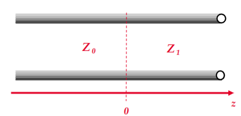
Quarter-Wave Transformer – The Impedance Viewpoint

The quarter-wave transformer is a transmission line segment of length used to match two impedances.

Input Impedance at :

The impedance transformation equation is given by:

Special Case for a Quarter-Wavelength Line:

Since the phase shift for a quarter-wavelength section is:

The input impedance simplifies to:

Transmission line length:

Condition for Perfect Matching:

To achieve impedance matching (), we set:

This ensures that all power is transferred to the load without reflections.

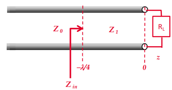
quarter wave transformer:




where
Thus, , so:

In our case, is close to 0, meaning no reflection.

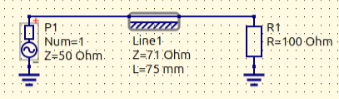
Lossy quarter wave transformer:

Smith chart

Topic: Transmission Lines
The scariest thing you learn in Electrical Engineering | The Smith Chart - YouTube

• When there is very high frequencies on small length it causes reflections, good example in the video with a pulsating rope.
• Smith chart shows how much Voltage transmitted vs how much is reflected.

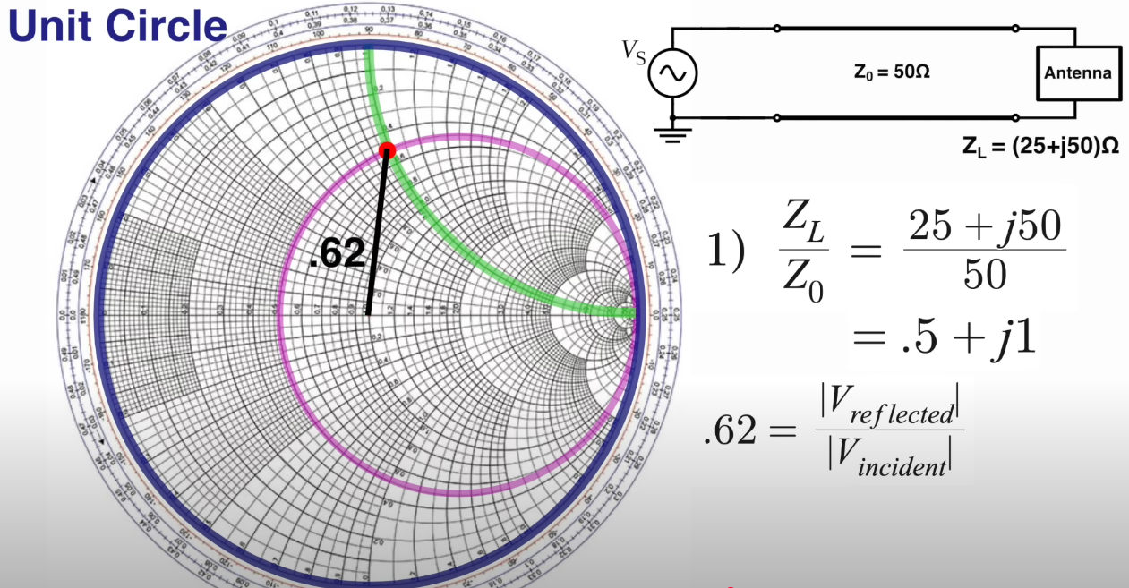
if the original signal is 10V then the reflection is 6.2V.




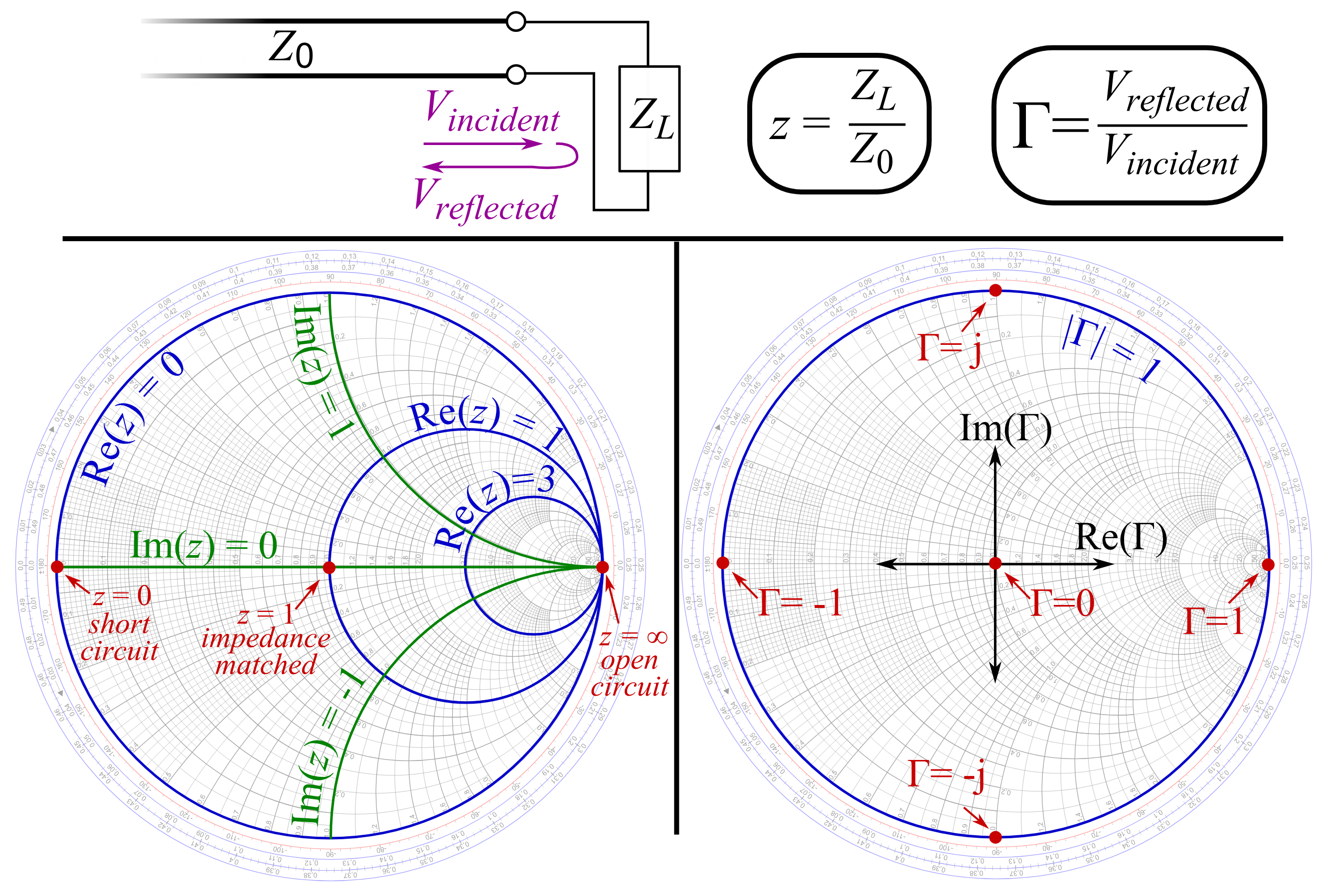
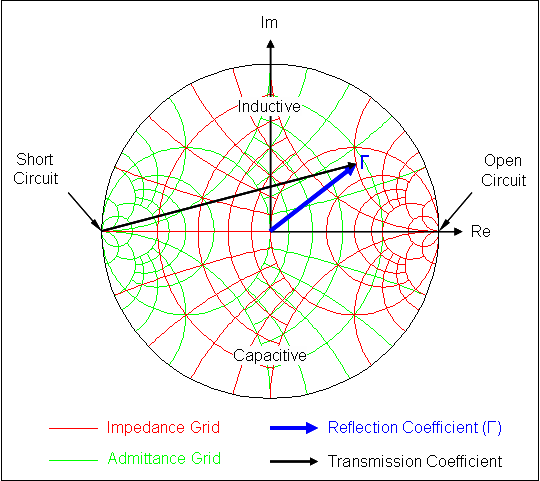
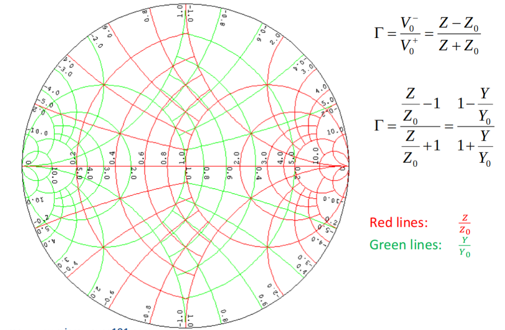
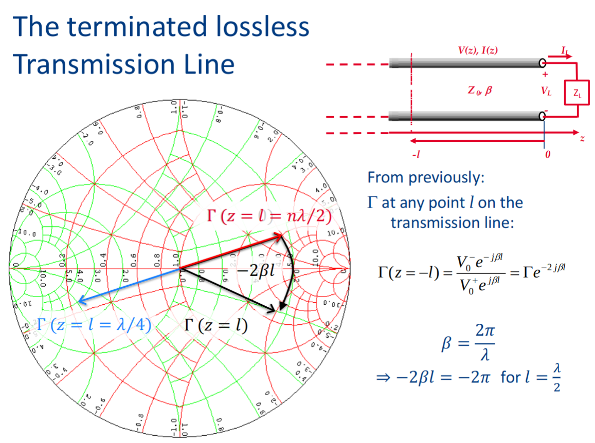
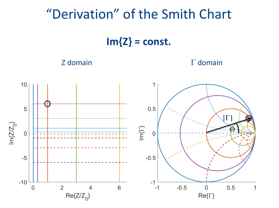
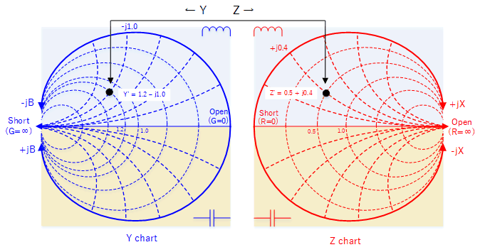
In the center it is the Load

finding reflection coefficient on smith chart
moving towards generator on smith chart

Passive microwave networks

5XTC0_Lecture_Module2_Passives.pdf

Formulas

Telegrapher’s Equations (frequency domain)

Voltage and Current in Transmission Line

Reflection Coefficient

Voltage and Current using

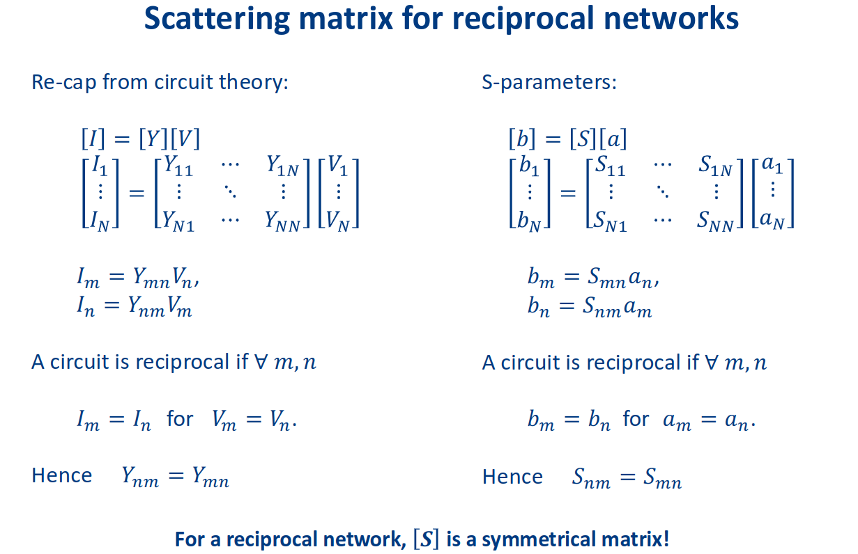
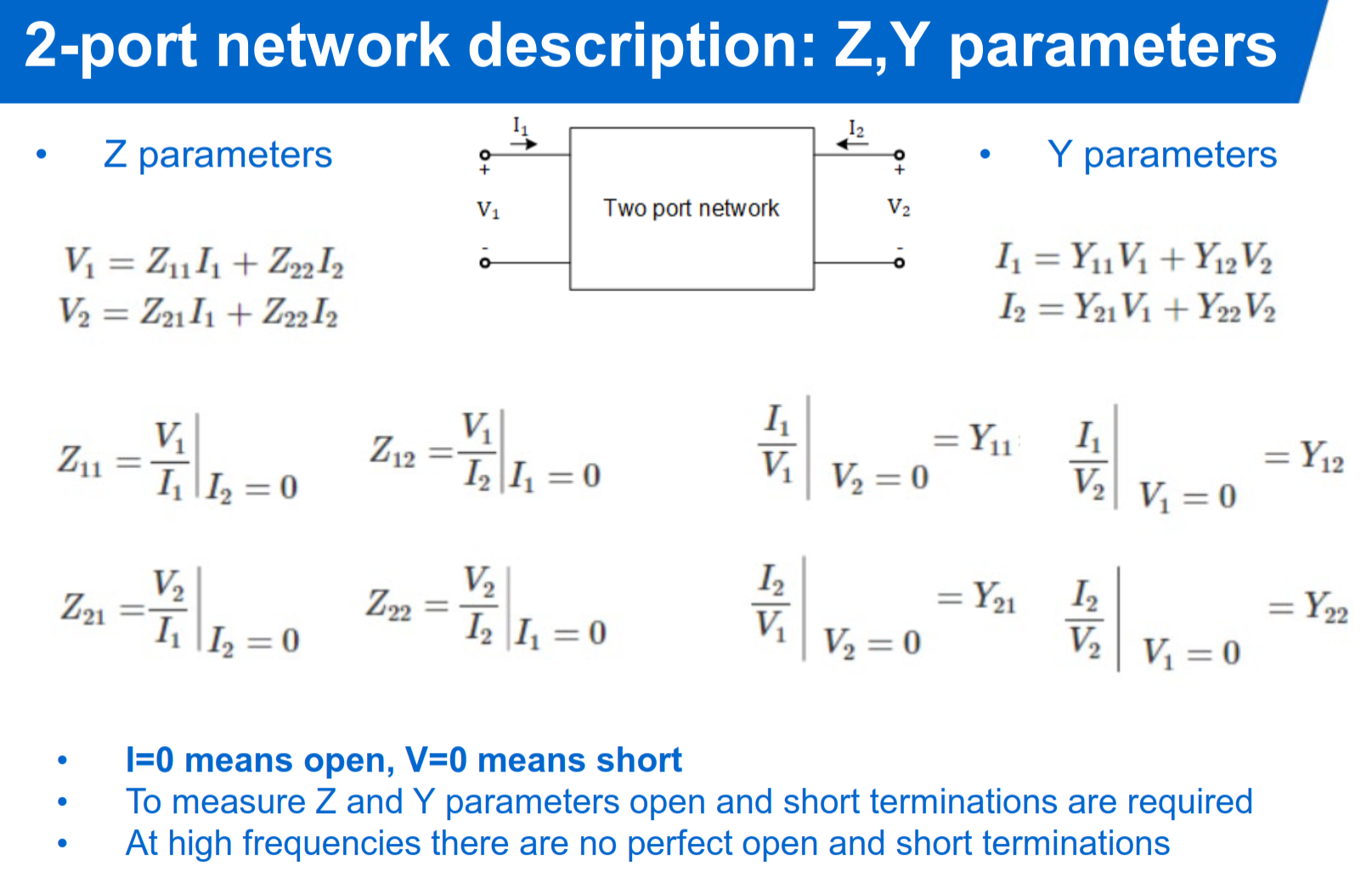
Impedance Matrix

Admittance Matrix

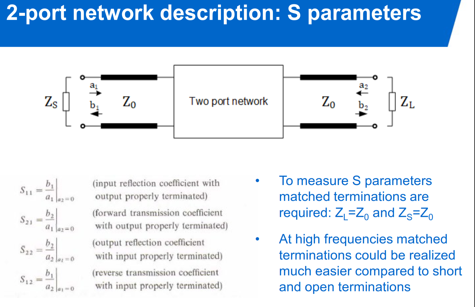
Scattering Parameters

Power at a Port

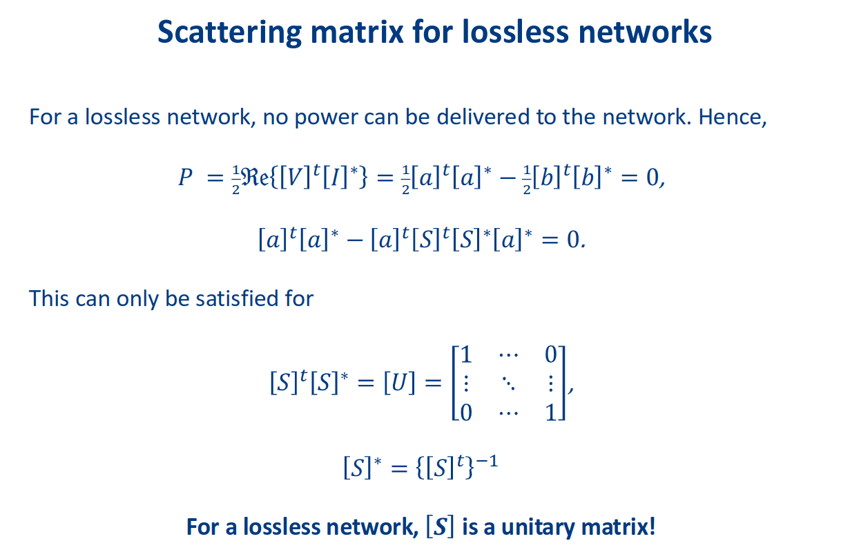
Unitary Condition (Lossless S-matrix)

Reciprocal Network (S-matrix Symmetry)

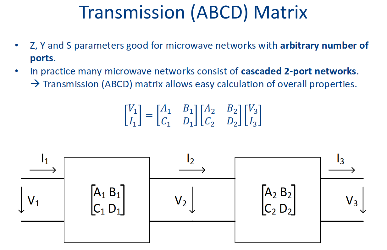
ABCD (Transmission) Matrix

Impedances of Lumped Elements (Series)

Admittances of Lumped Elements (Parallel)

Quarter-Wavelength Transformer

Transmission Line Impedance Transformation

Power Divider (Asymmetrical)

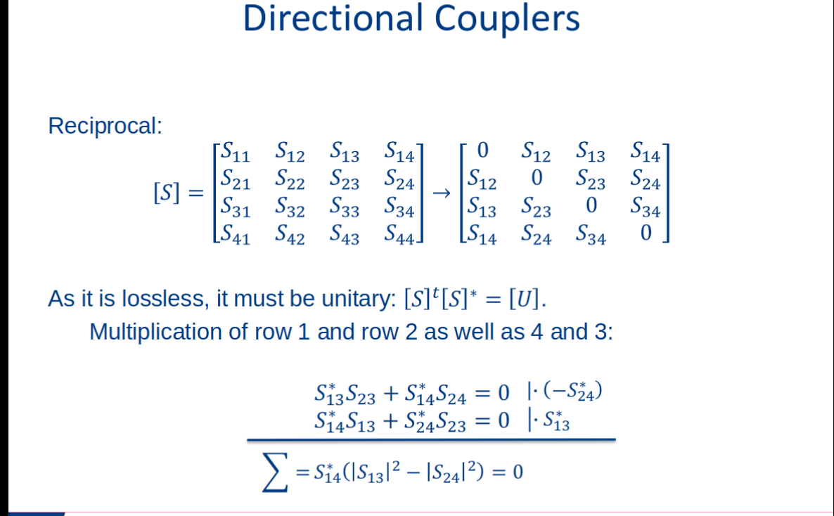
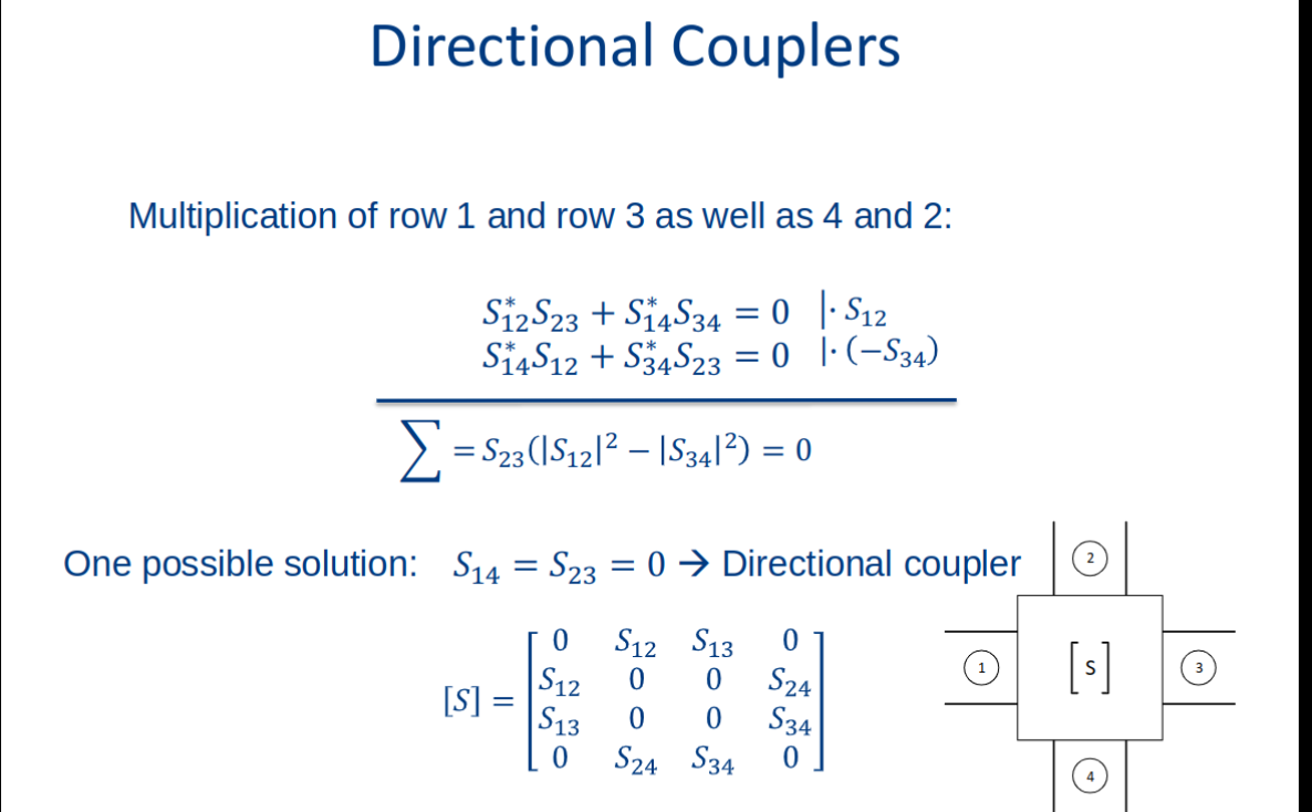
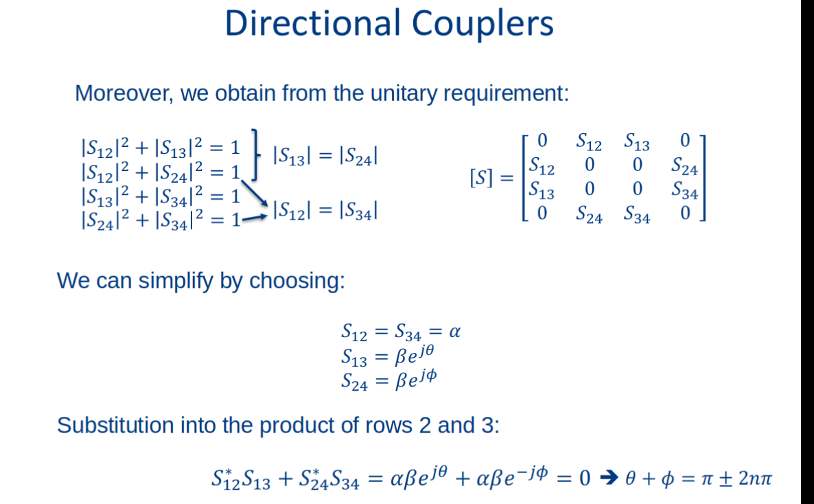
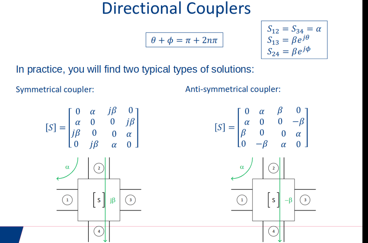
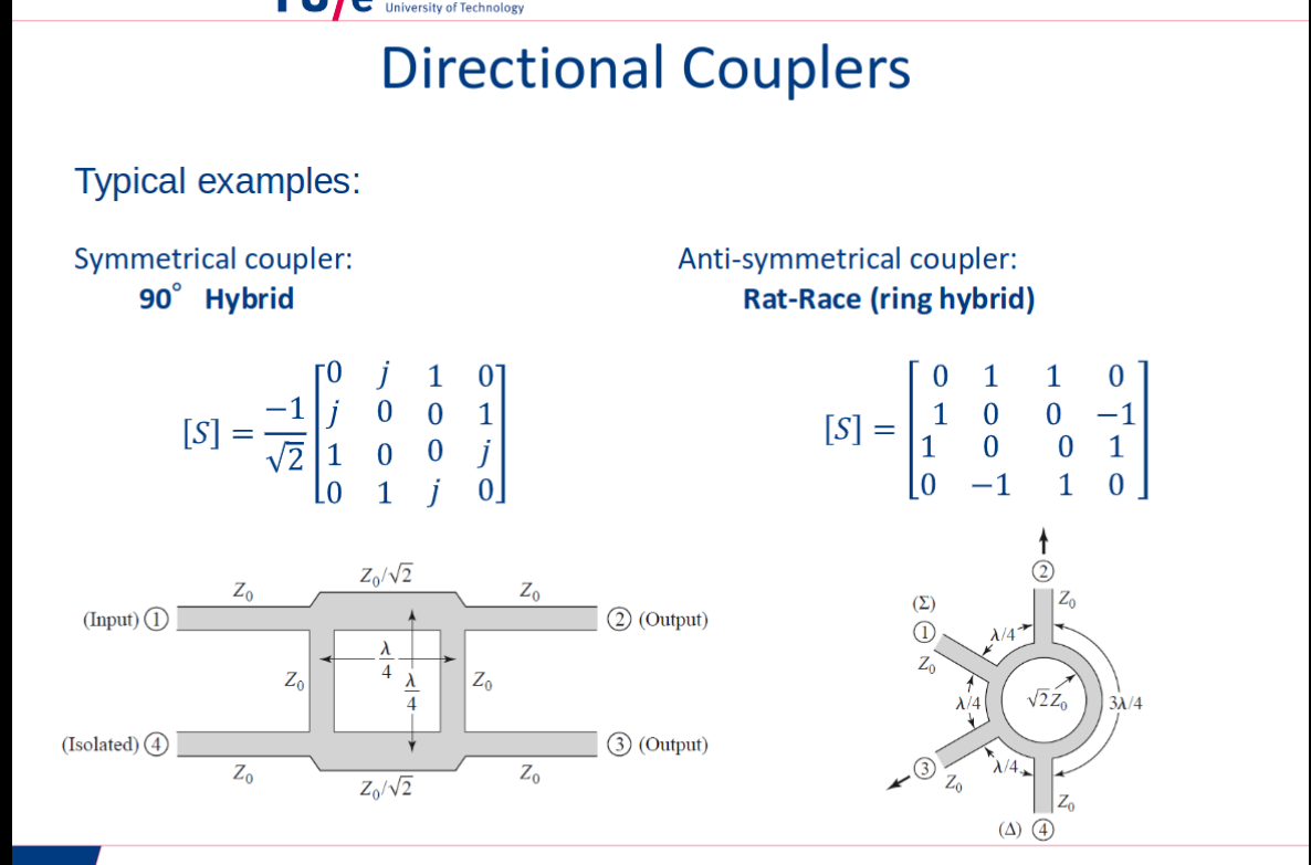
Directional Coupler (Symmetrical)

Directional Coupler (Anti-symmetrical)

Microwave network matrices

Topic: S-Parameters and Impedance Matching
and

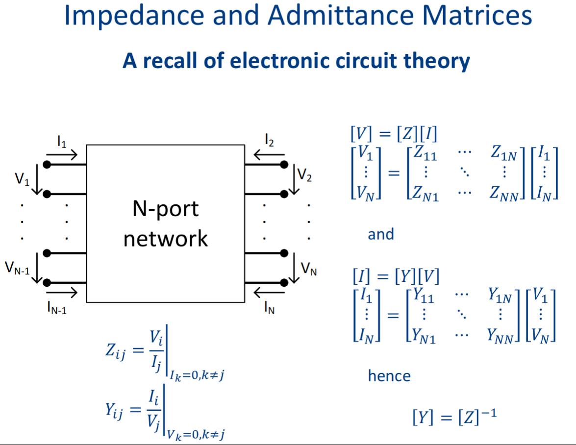
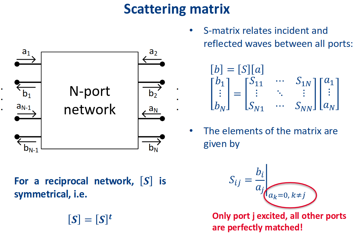
microwave circuits:

• Voltage and current difficult to measure (either separate measurement of and or of standing wave pattern required)
• Voltage and current difficult to define for non-TEM transmission lines.

Scattering parameters

using power relations: wave amplitudes defined to obtain meaningful power relations: knowing the microwave circuit equations of
power delivered to port = incident - reflected wave

Impedance matching and tuning

Topic: S-Parameters and Impedance Matching

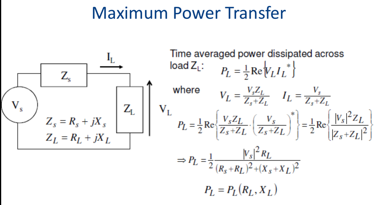
letting we fine that value to max the power transfer to load impedance must be complex conjugate of this is called Conjugate Matched.

Matching Network

normalizing impedance for smith chart:
de-normalizing (real impedance):
normalized impedance:

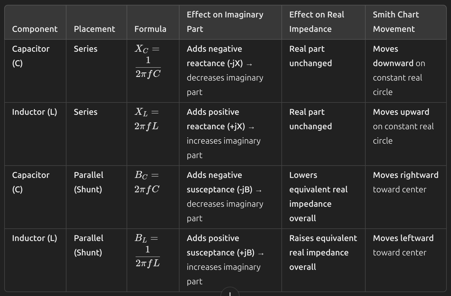
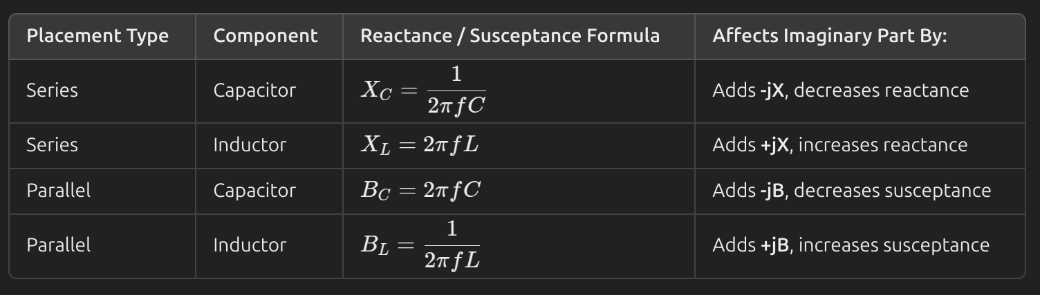
Impedance matching network

such network is pushed between source and load in the case there are reflections due to , in the course we only deal with single frequencies but in general the impedance matching network can range for Broadband.

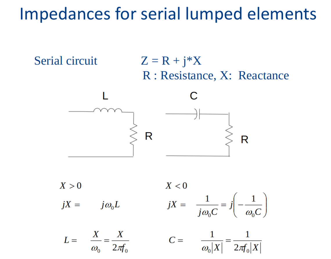
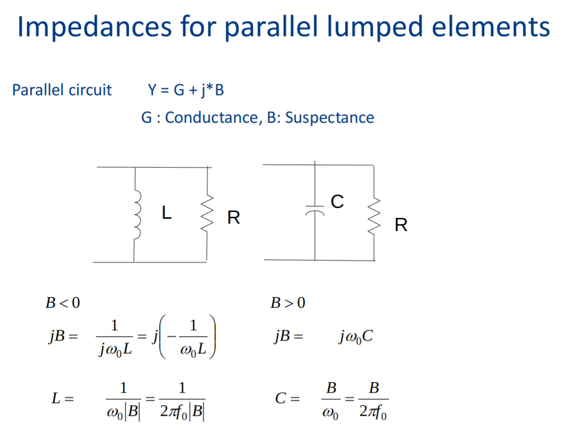
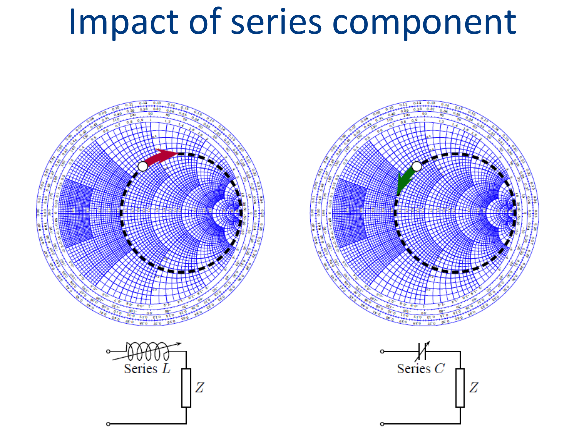
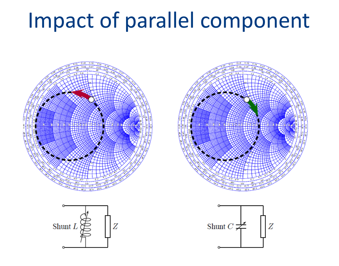
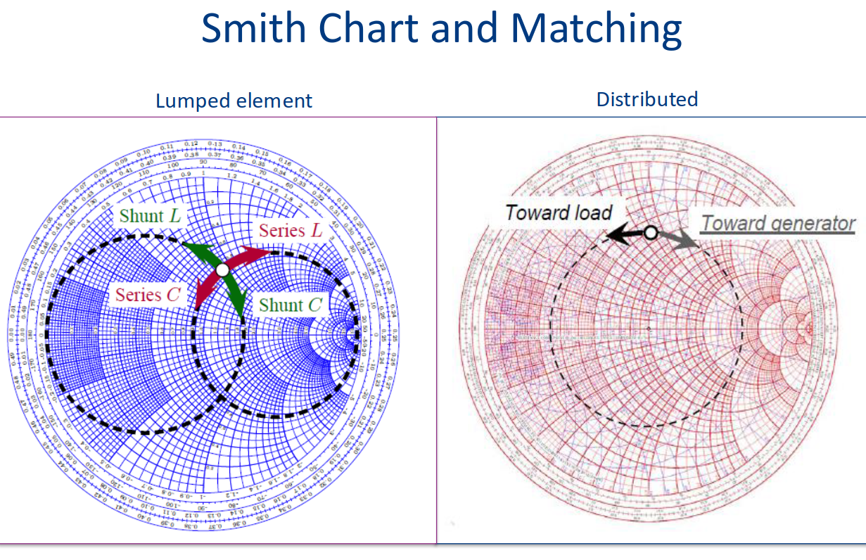
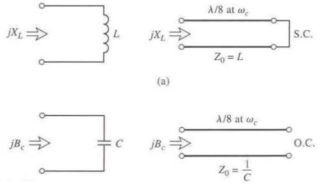
Distributed elements (using stubs to mimic lumped components)

inductances and capacitances can be achieved using transmission lines:

Inductance:
Capacitance:

Power dividers and directional couplers

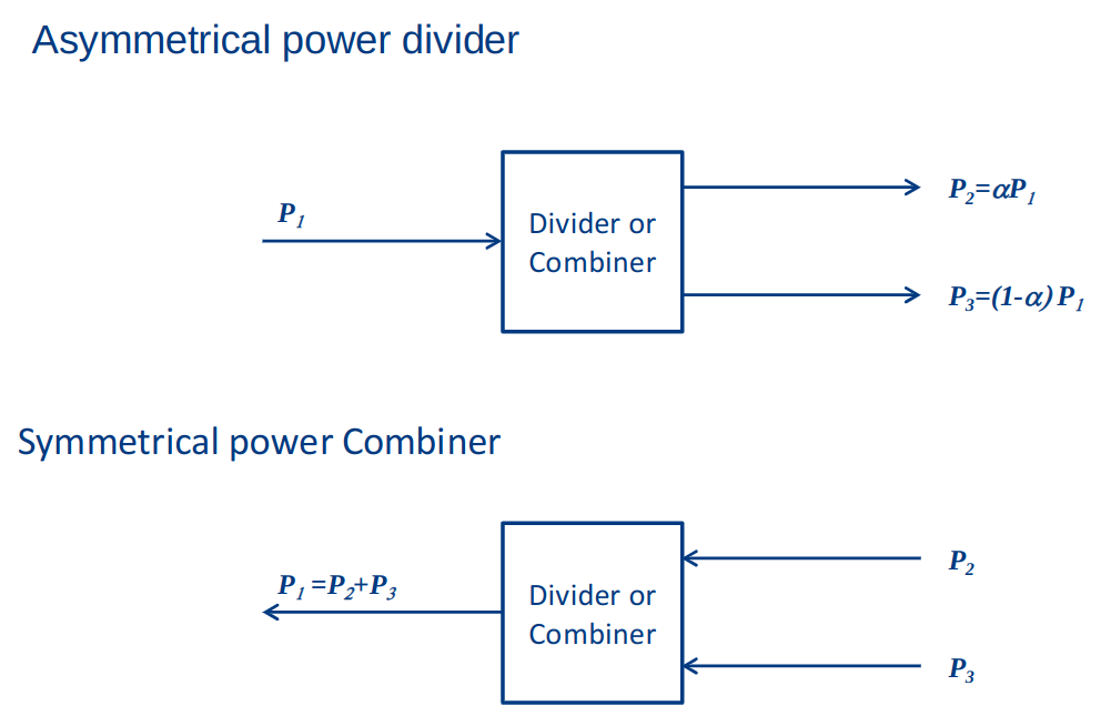
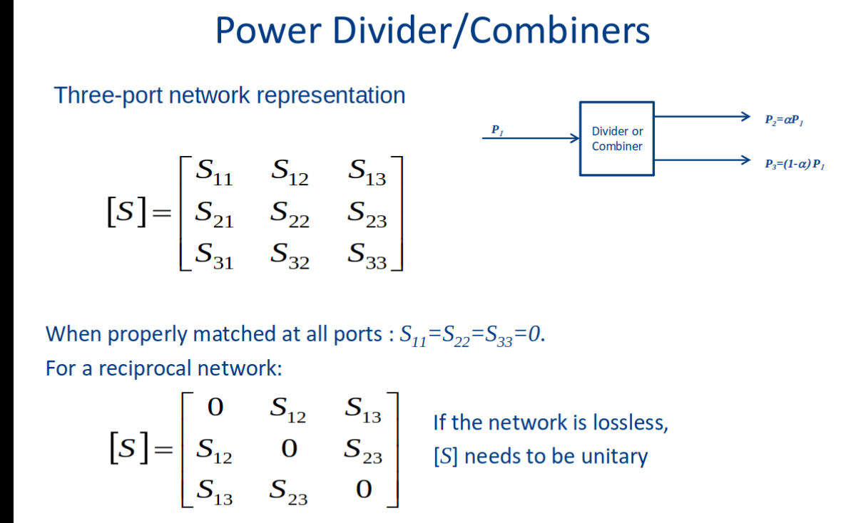
A power divider network can have symmetrical or asymmetrical.

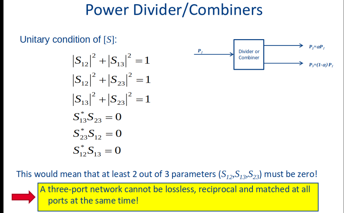
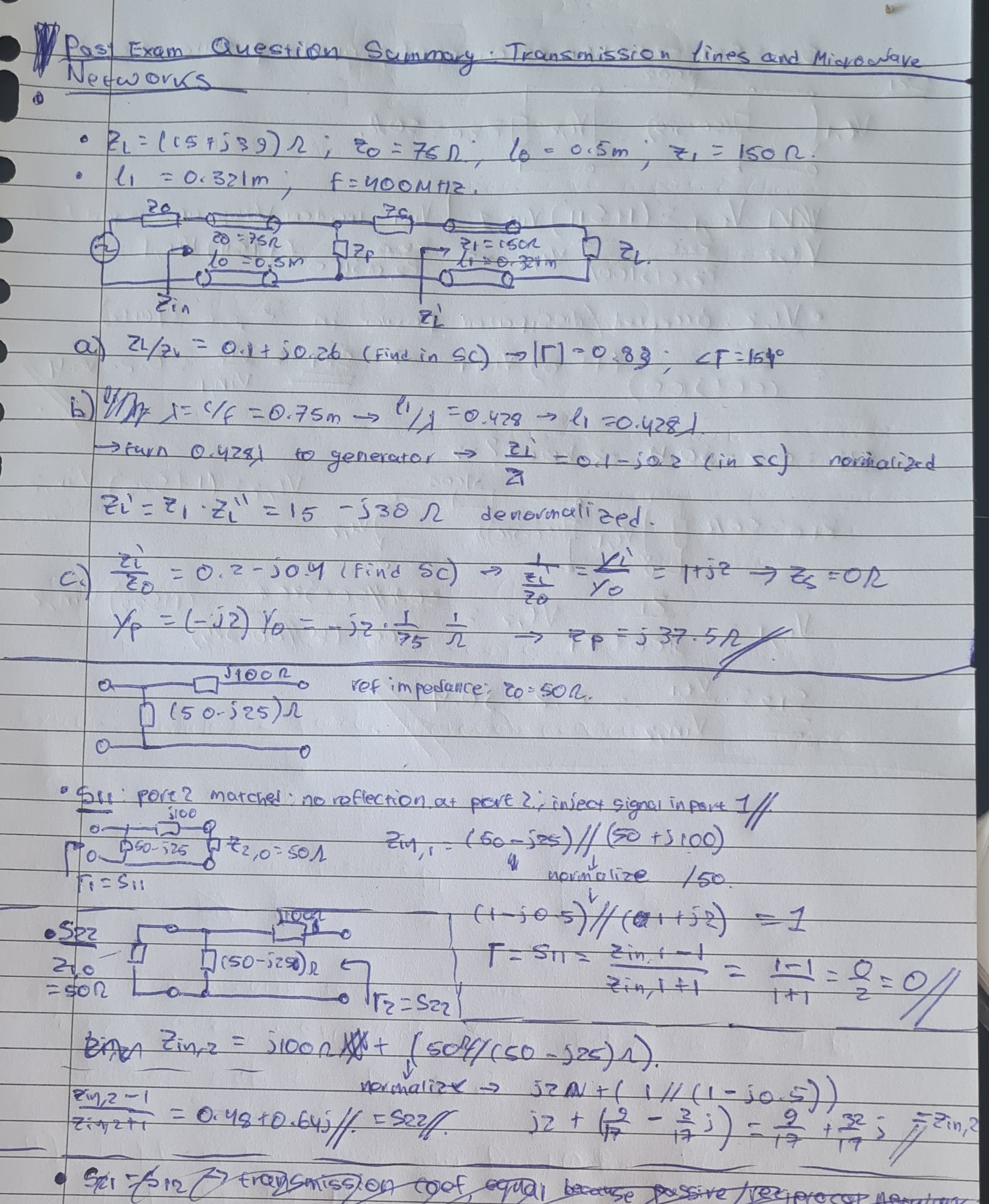
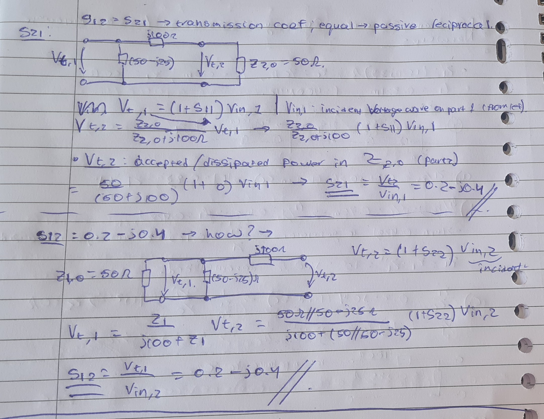
Matrix Based Question

Antenna parameters & theory

Topic: Antennas and Radiation

5XTC0_Lecture_Module3_Antenna-Parameters-3.pdf

Formulas

Poynting Vector (Instantaneous):

Time-Averaged Power Density:

Radiation Intensity:

Surface Element in Spherical Coordinates:

Solid Angle:

Total Radiated Power:

Directivity:

Gain:

Gain vs Directivity:

Reflection Efficiency:

Axial Ratio (AR):

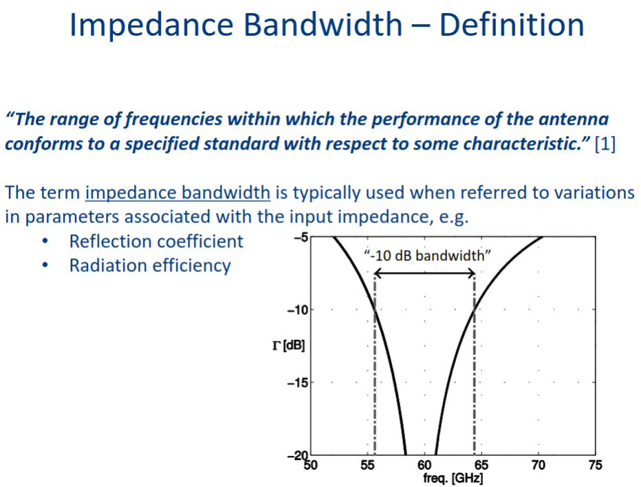
Bandwidth:

Narrowband Percentage:

Input Impedance (Thevenin Model):

Input Admittance (Norton Model):

Radiation Efficiency (Power-Based):

Received Power and Effective Aperture:

Effective Aperture:

Max Effective Aperture (Matched Case):

Free Space Power Density:

Max Effective Aperture (Dipole Example):

Friis Transmission Equation:

Gain-to-Aperture Relationship:

Radiation parameters

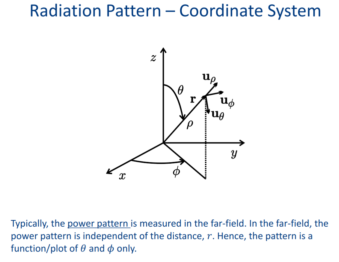
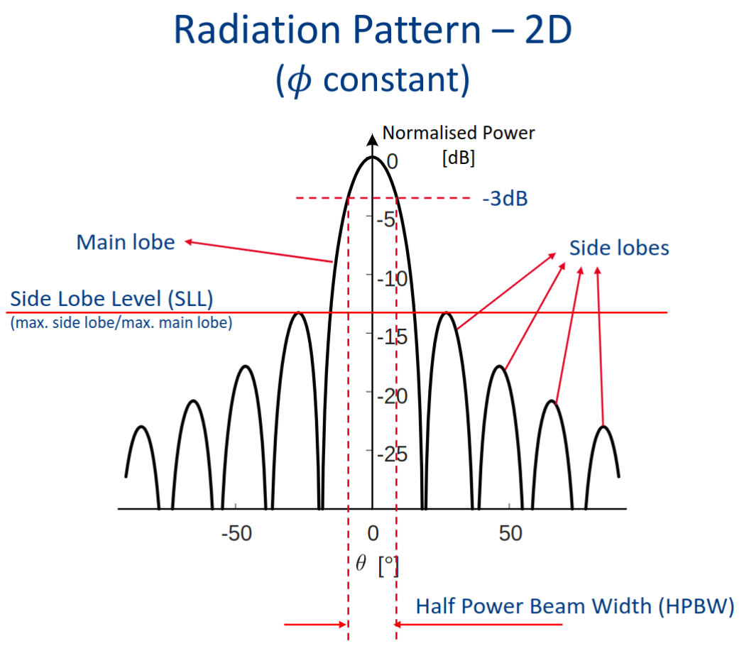
Radiation Pattern

spatial distribution of quantity that characterizes the electromagnetic field generated by an antenna.

The distribution can be expressed as mathematical function as graphical representation.

when the amplitude or relative amplitude of a specified component of the electric-field vector is plotted graphically, it is called an amplitude pattern, field pattern or voltage pattern. When the square of the amplitude or relative amplitude is plotted, it is called a power pattern.

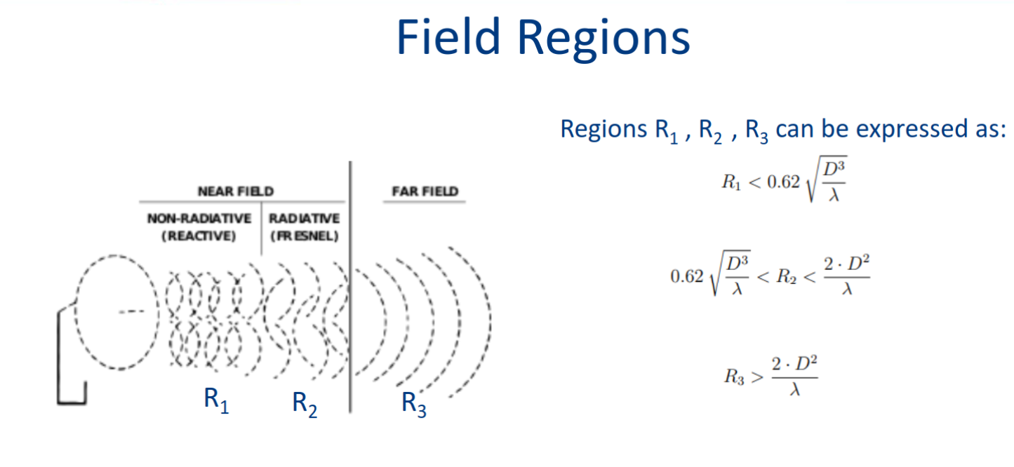
• Reactive near-field region:

• Reactive fields predominate

• Radiation pattern changes with

• Radiating near-field (Fresnel) region:

• Radiation fields predominate

• Radiation pattern changes with

• Far-field (Frauhofer) region:

• Radiation fields predominate

• Radiation pattern independent of

Near and far field - Wikipedia

Poynnting vector: .

The power density decays with hence the radiation intensity is defined as distance independent parameter, provides radiated power per unit solid angle.

To have power independent figure we normalize the radiation intensity with respective radiation intensity of (ideal) isotropic radiator: where is directivity. and isotropic radiator: .

To know the directivity radiated power is needed, we obtain gain: the input power is related to radiated power by efficiency: so

Directivity - Wikipedia

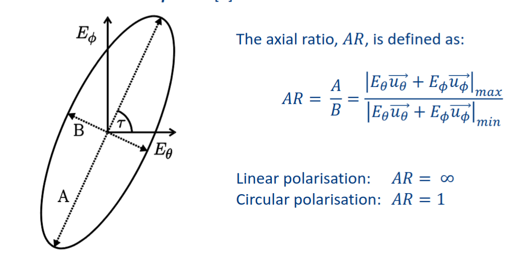
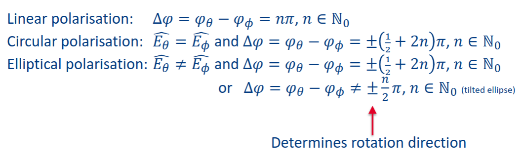
Polarization

In a specified direction from an antenna and at a point in its far field, the polarization of the (locally) plane wave that is used to represent the radiated wave at that point.

wave propagating towards , and its electric field can be decomposed in time domain:

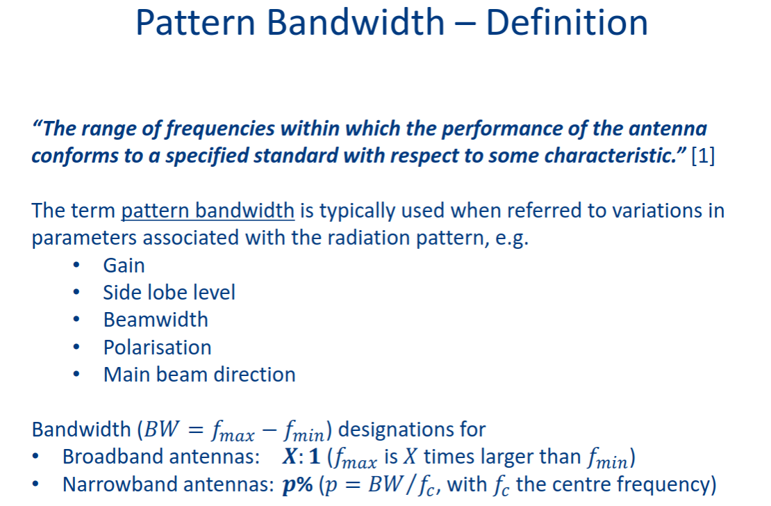
Circuit level representation

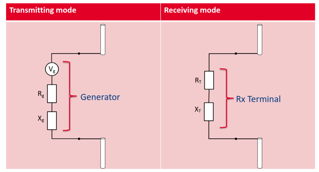
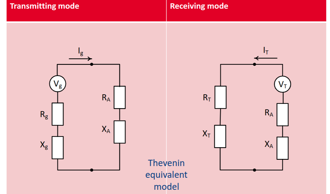
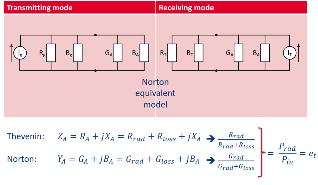
In receive mode the power accepted by Rx terminal can be linked to power density, of the incident electromagnetic wave: where is effective aperture of antenna. and for max power transfer:

Propagation channel basics

Topic: Wireless Channel
The Friis transmission equation relates the power received by an antenna 2 to the radiated power by antenna 1 and vice versa.

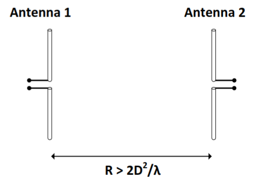
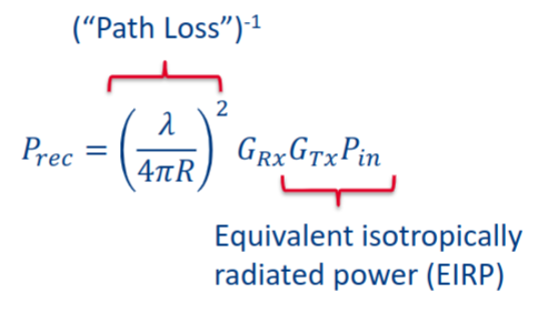
The power density of isotropic radiator at distance is given by: , so for real antenna: .

power received by antenna 2 depends on its effective aperture: so if antenna 2 was in transmitting mode and antenna 1 as receiving antenna, we get: hence: .

Ratio of gain to effective aperture in certain direction is same for all antennas, for example for very short dipole , max gain: 1.5 so so rewriting for received power: .

Friis Transmission equation:



Friis transmission equation - Wikipedia

FSPL - Free Space Path Loss: influenced by frequency operation - Friis equation → has a wavelength component.

RF systems and Amplifier design

5XTC0_Module_4_Amplifier_Design.pdf

5XTC0_Module_4_RF_Systems.pdf

Formulas

Reflection Coefficients

Input and Output Reflection Coefficients

Power Calculations

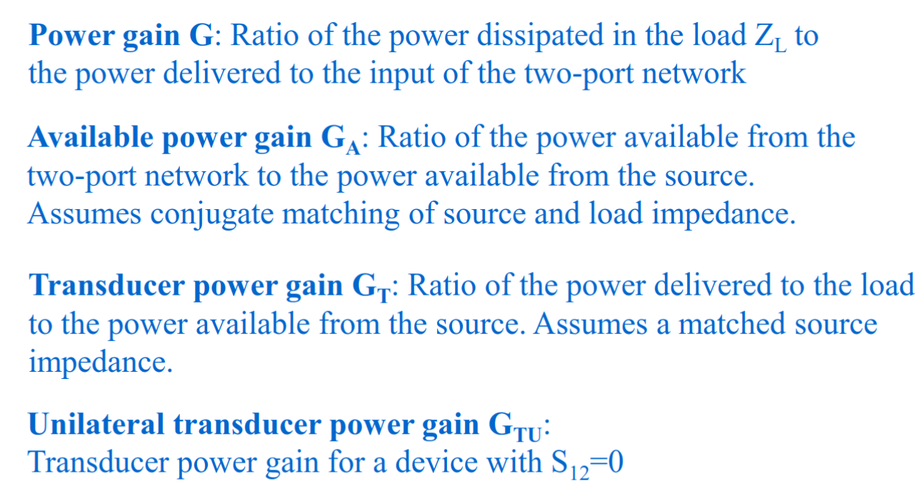
Power Gains
Power gain:
Available power gain:
Transducer gain:
Unilateral transducer gain (S₁₂ = 0):

Gain Circle Parameters
Normalized gain factor:
Center:
Radius:

Stability Factor and Condition
Rollet stability factor:


Condition for unconditional stability:
and

Stability Circle Centers and Radii
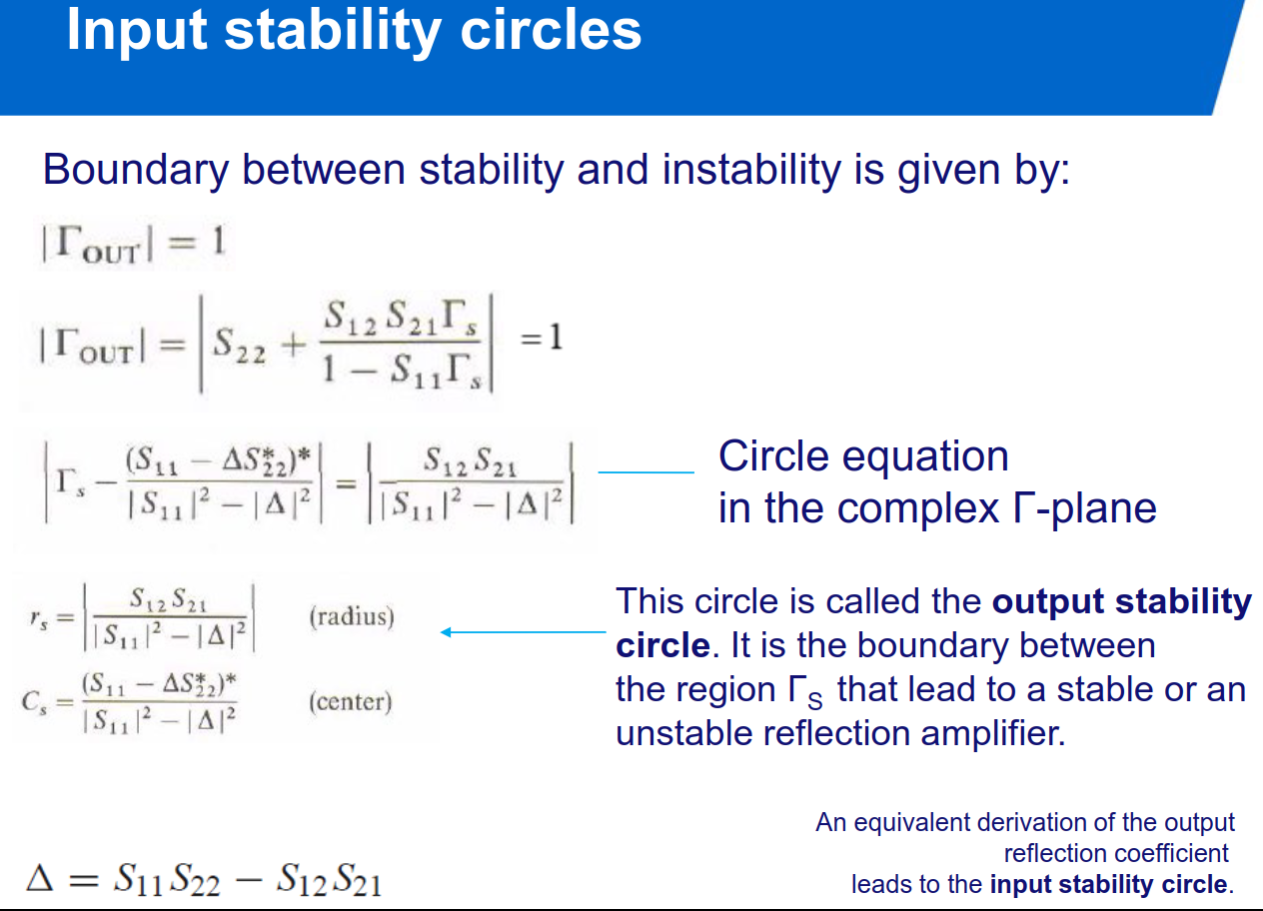
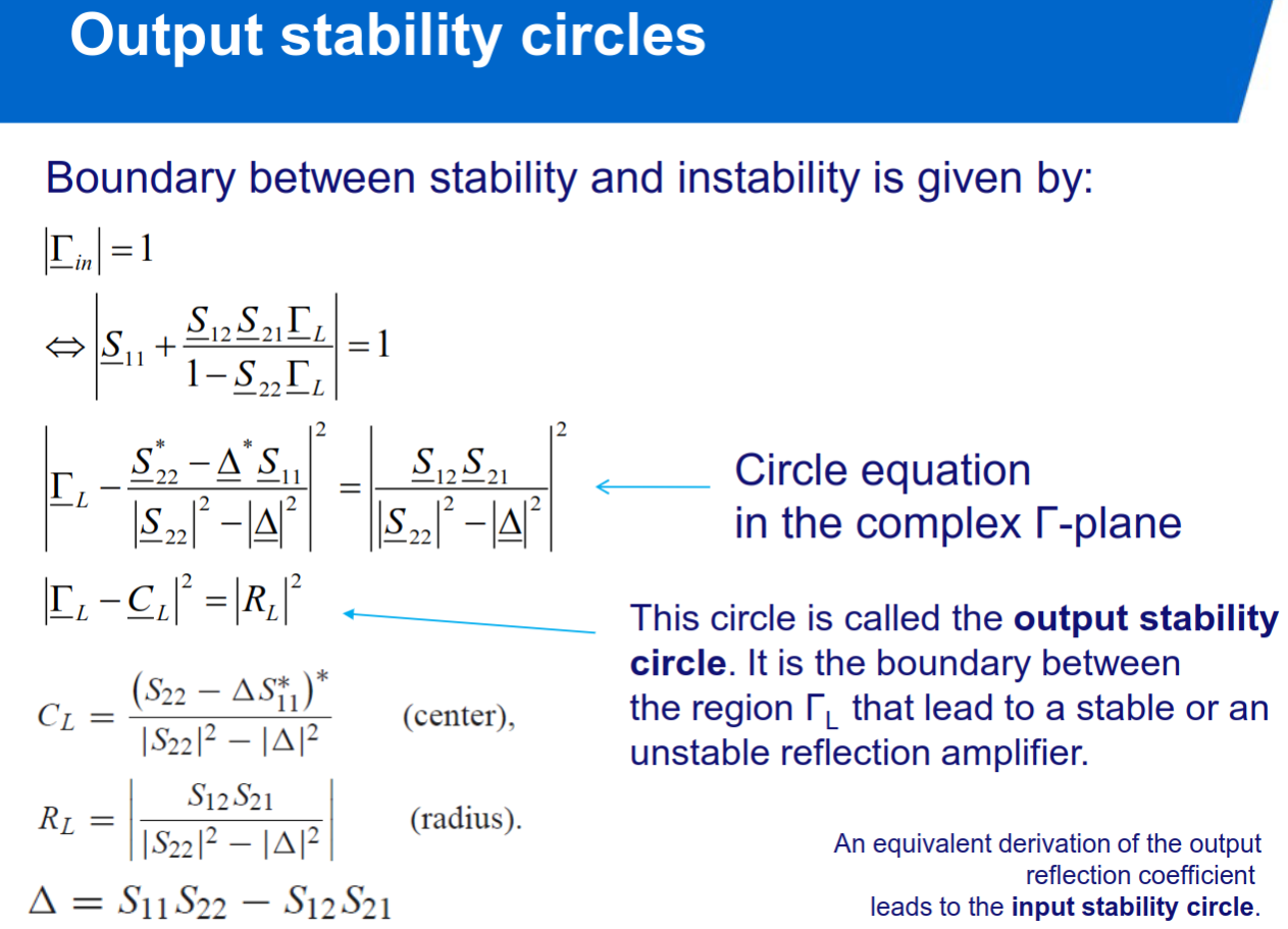
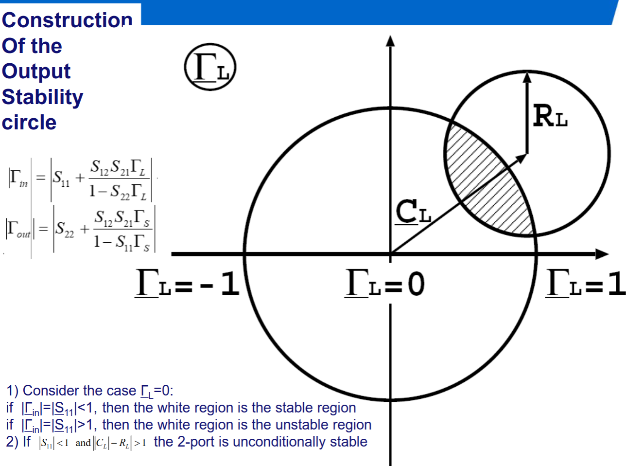
Input stability circle (in Γ_L plane):

Output stability circle (in Γ_S plane):

RF systems

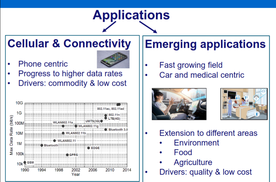
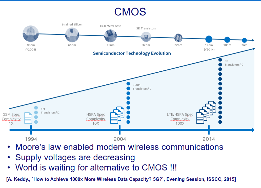
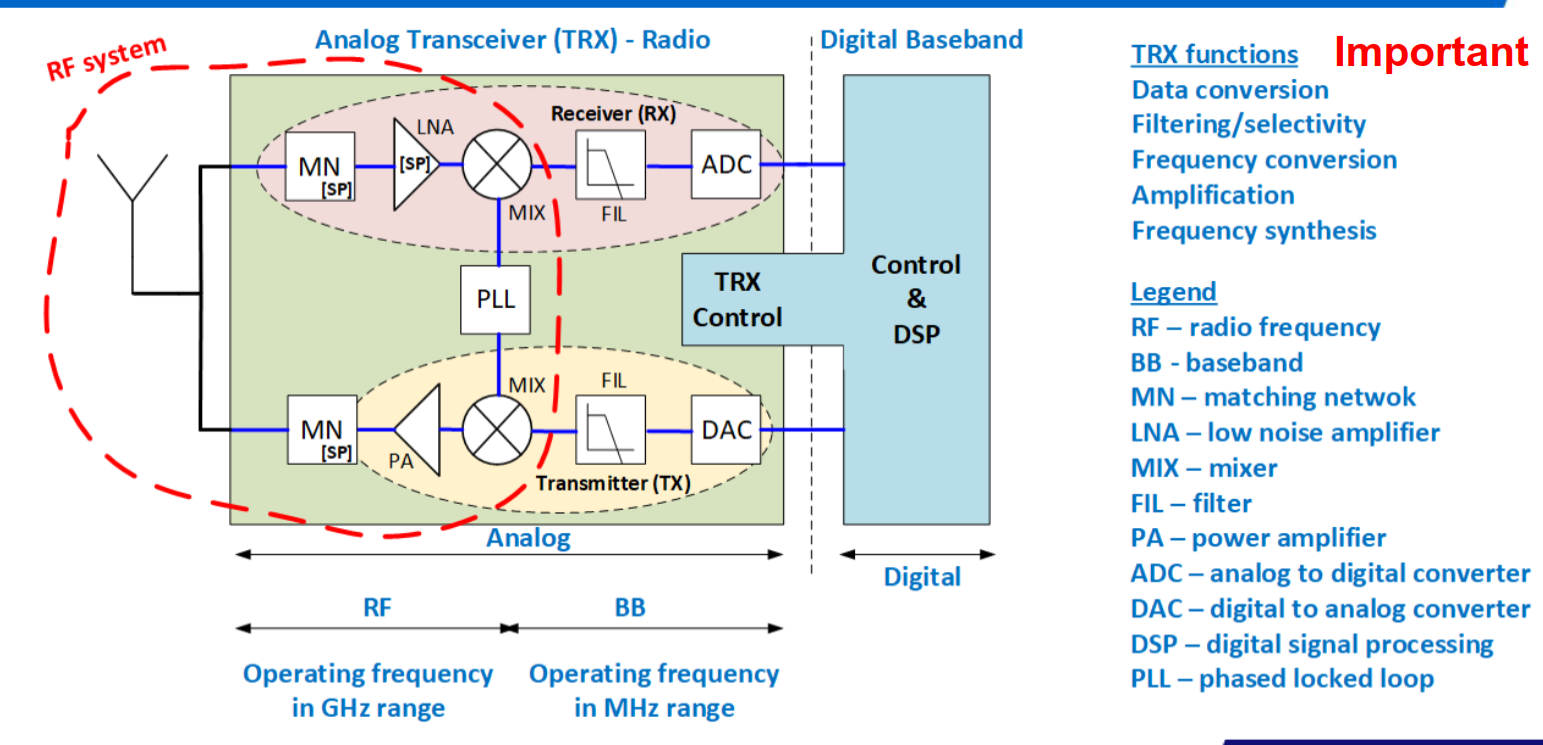
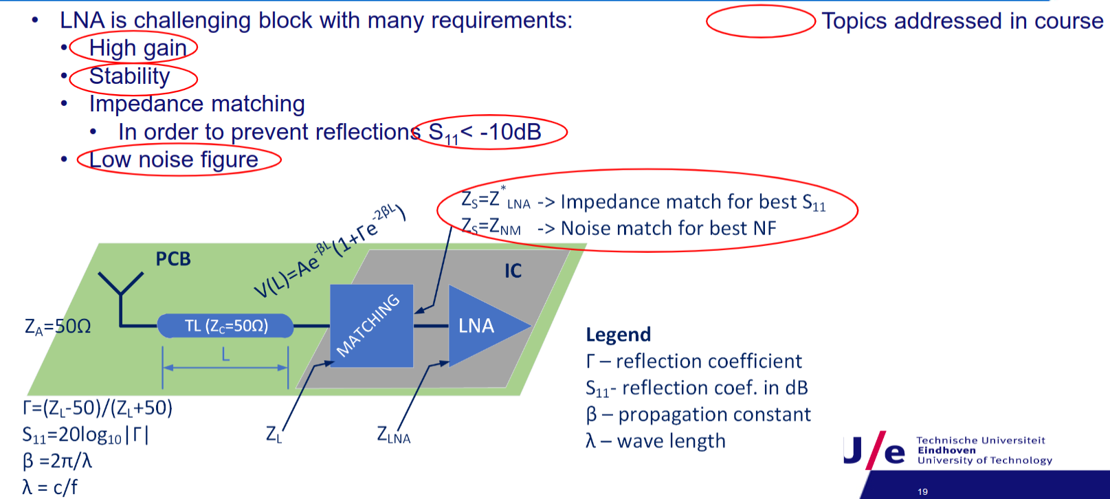
Amplifier design

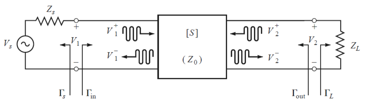
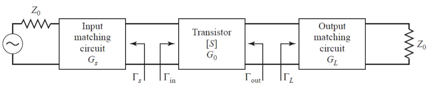
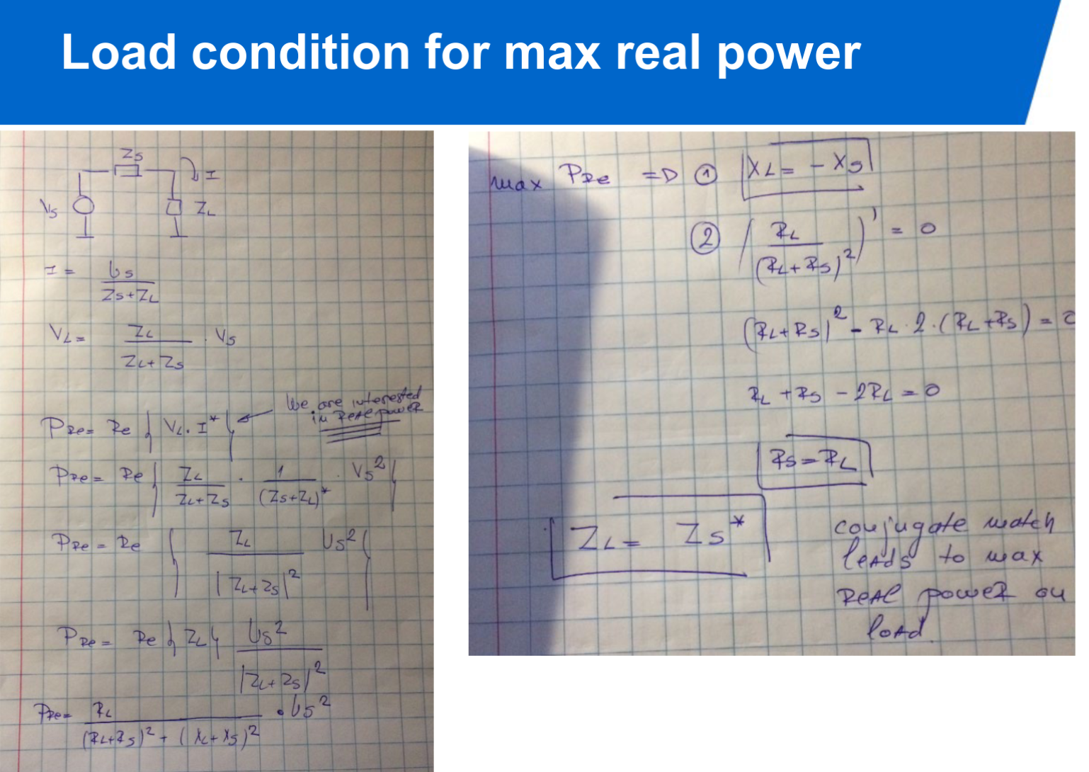
• Power available from source: , when source impedance is conjugately matched to input impedance: .
• Power available from network: , when load impedance is conjugately matched to output impedance: .

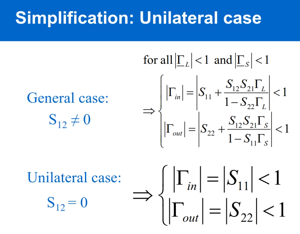
Unilateral Amplifier

An amplifier whose output exhibits no feedback to its input side is described as ‘unilateral’. The input impedance of a unilateral amplifier is independent of load, and output impedance is independent of signal source impedance.

, ,

If then: and

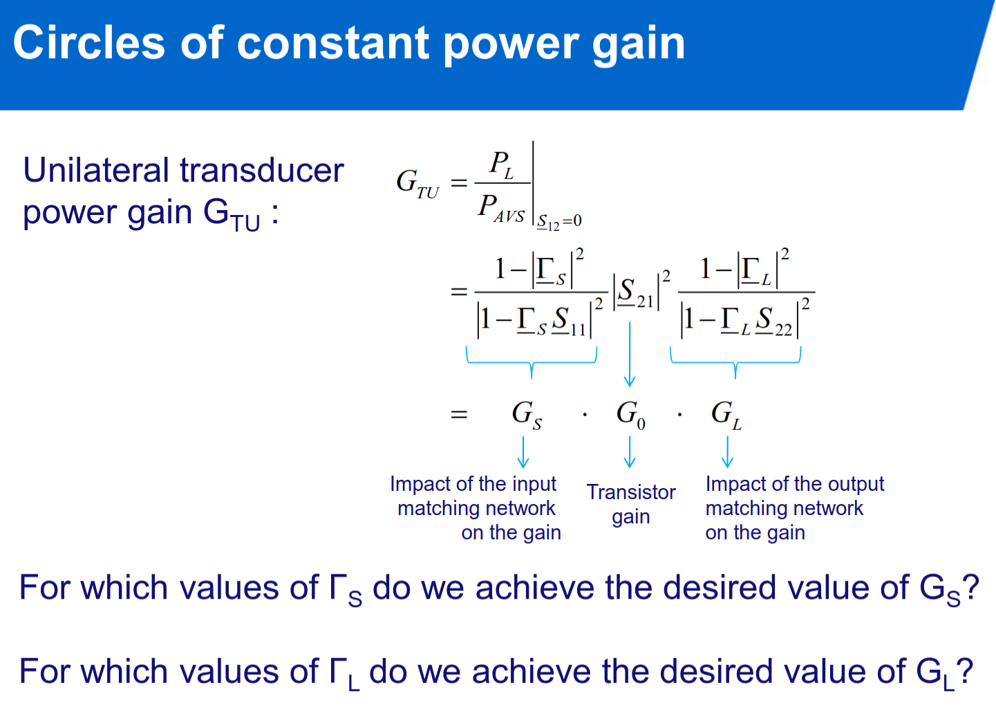
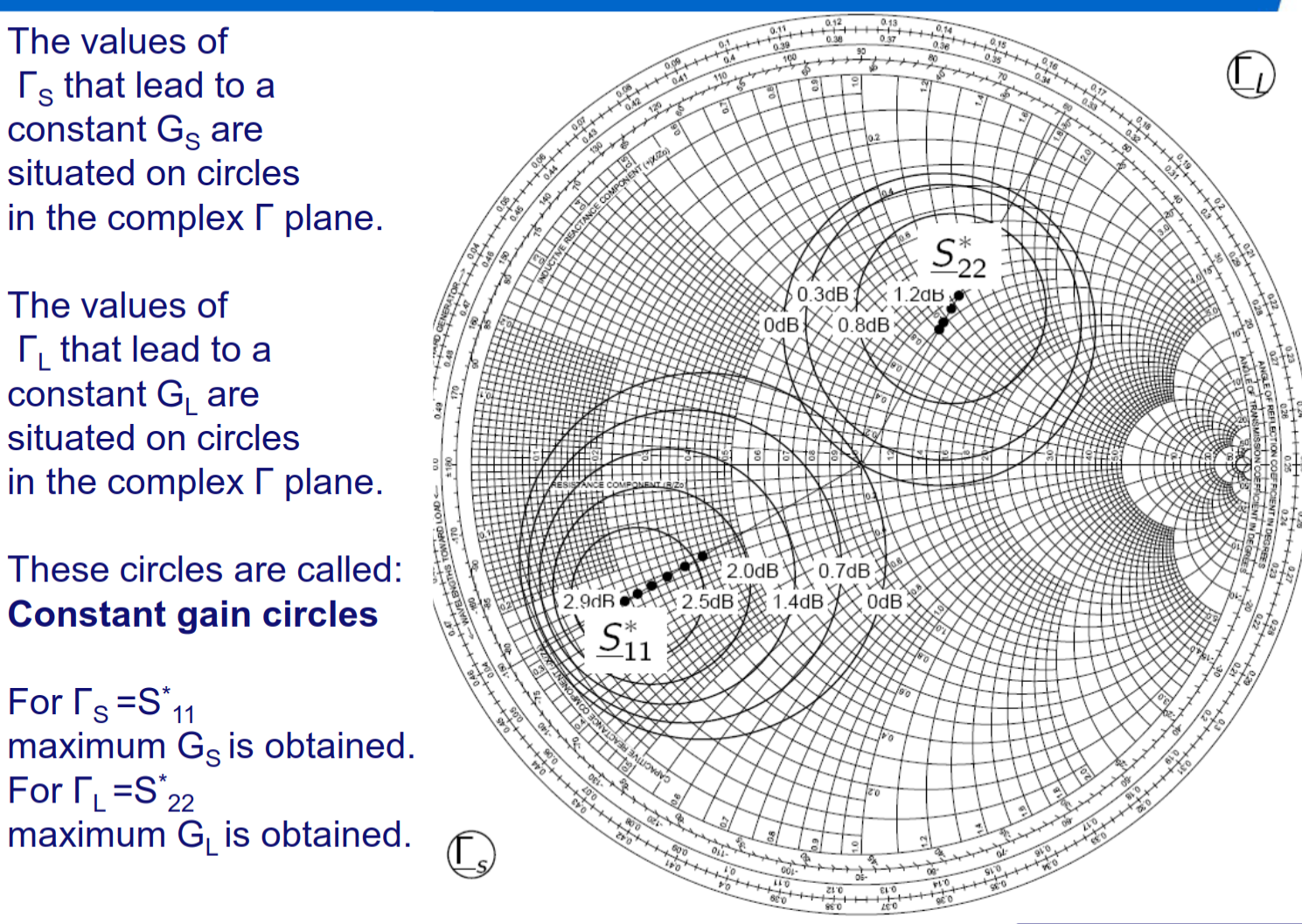
circles of constant power gain:
max gain of input and output matching networks:

normalized gain factors and :

center and radius of constant gain circle for input and output matching network:

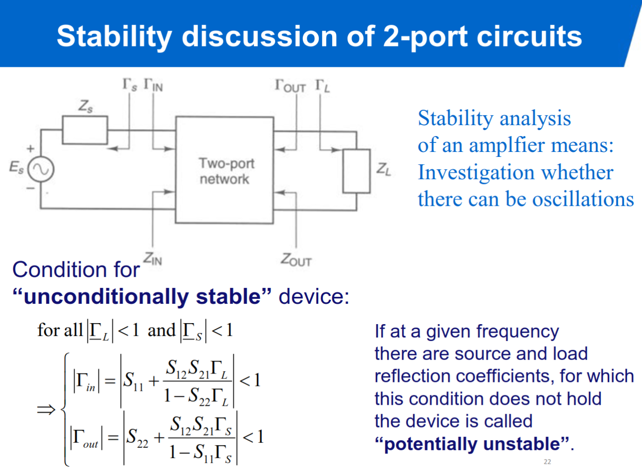
If than the 2-port is unconditionally stable. Unilateral case: , the conditions for unconditional stability: .
Where K is the Rollet stability factor.

Noise and LNA design

Topic: Noise
5XTC0_Module_5_Exercise_Amplifier_and_Low_Noise_Amplier_design.pdf

Formulas

Power Gain:

Available Power Gain:

Transducer Power Gain:

Unilateral Transducer Gain (S_{12}=0):

Reflection Coefficients: ,

Rollet Stability Factor: , with

Unconditional Stability Conditions: and

Thermal Noise Power:

Available Noise Power from Resistor:

Equivalent Noise Temperature:

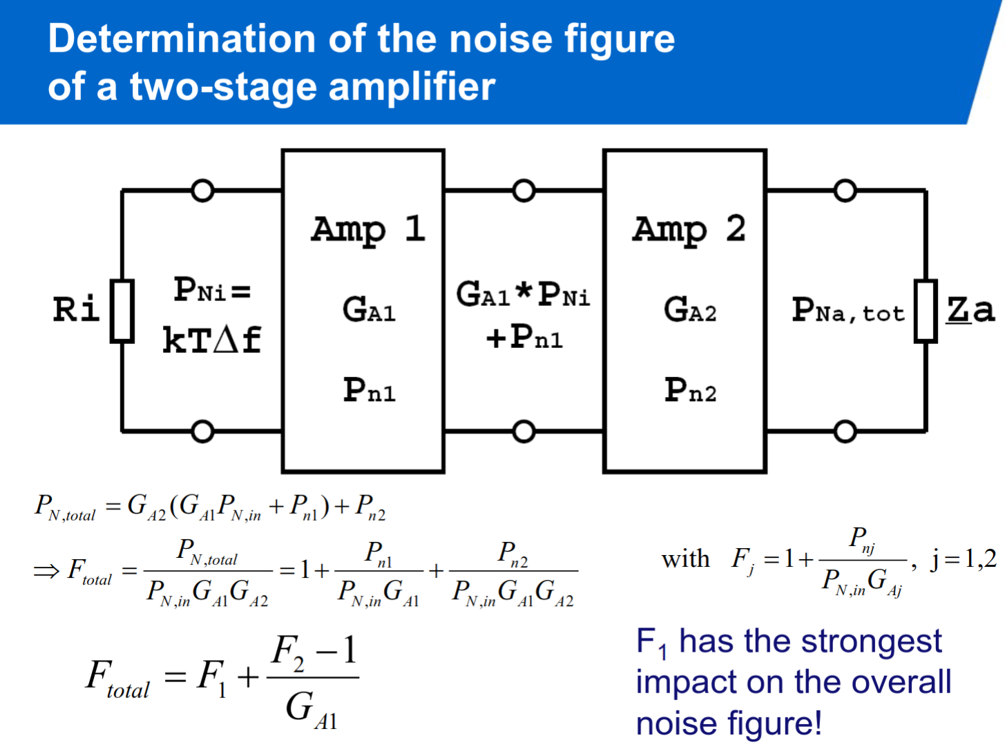
Noise Figure: , with

Friis’ Formula for Cascaded Stages:

Noise Figure with Source Admittance:

Noise Figure with Reflection Coefficients:

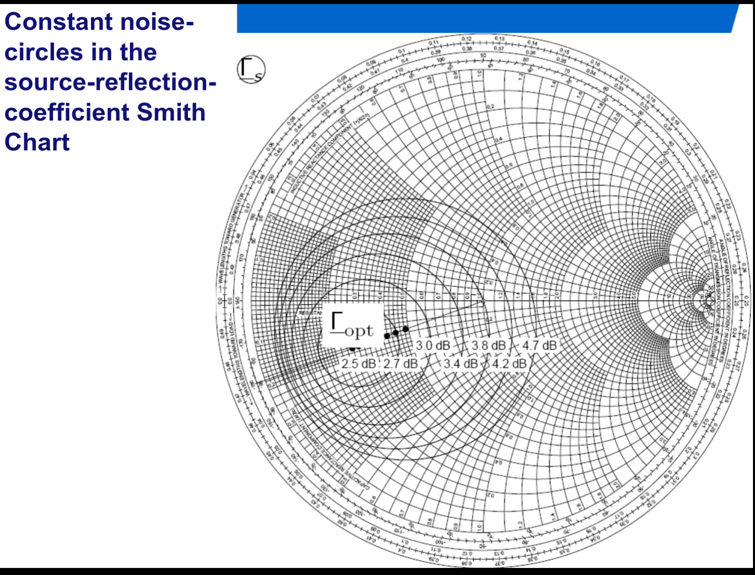
Constant Noise Circle Radius:

Constant Noise Circle Center:

Other

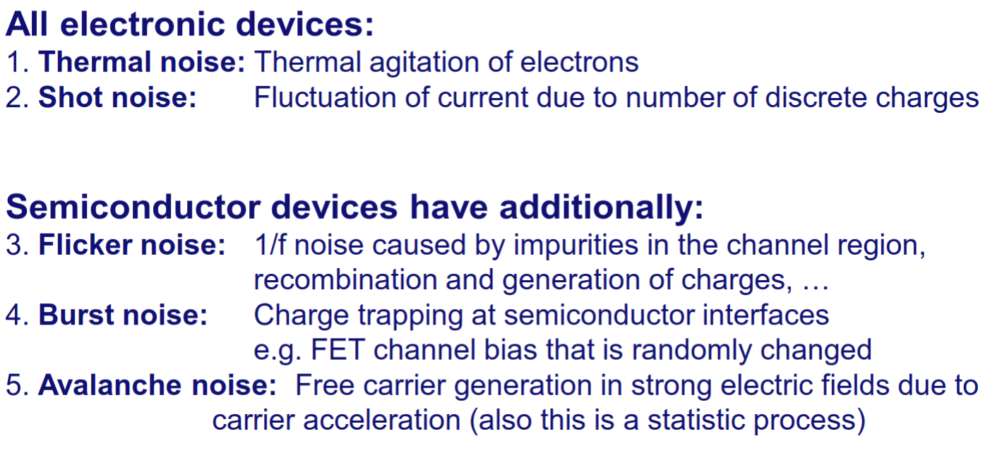
Thermal noise:
average voltage is zero, but non zero average power.

White noise:

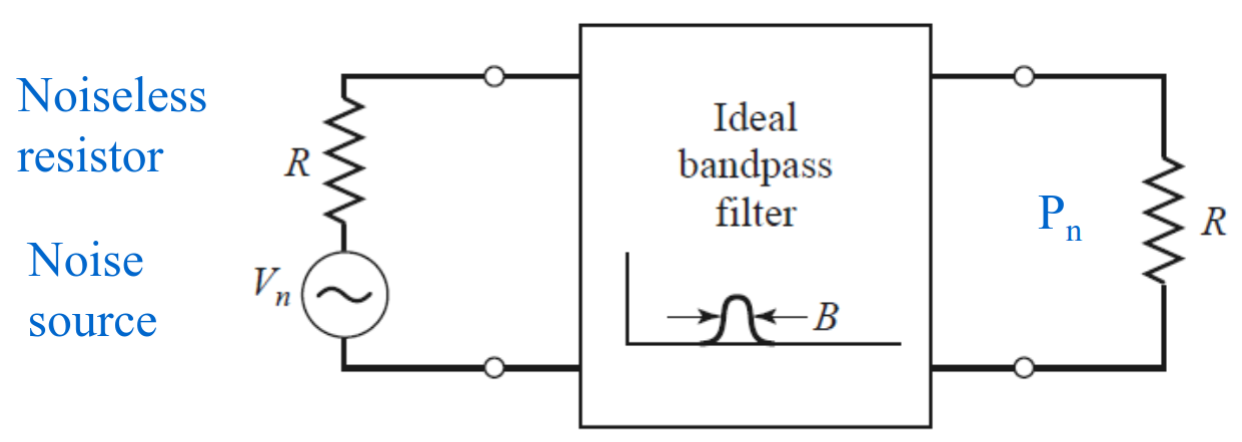
Noise of arbitrary source:

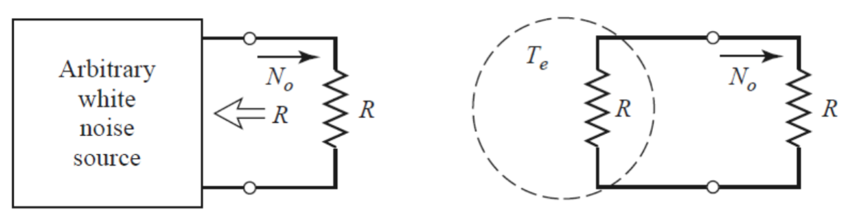
equivalent noise temperature:

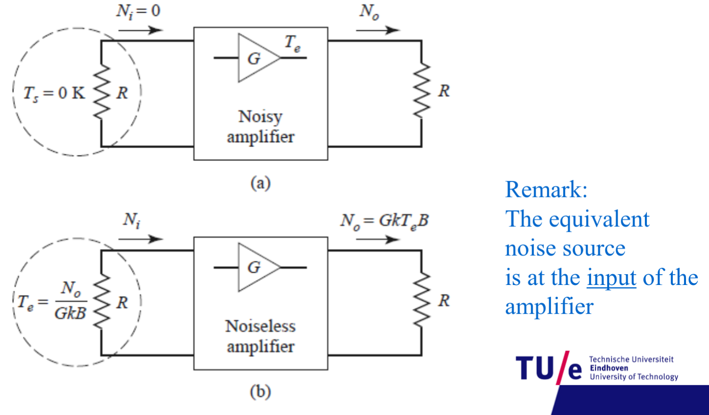
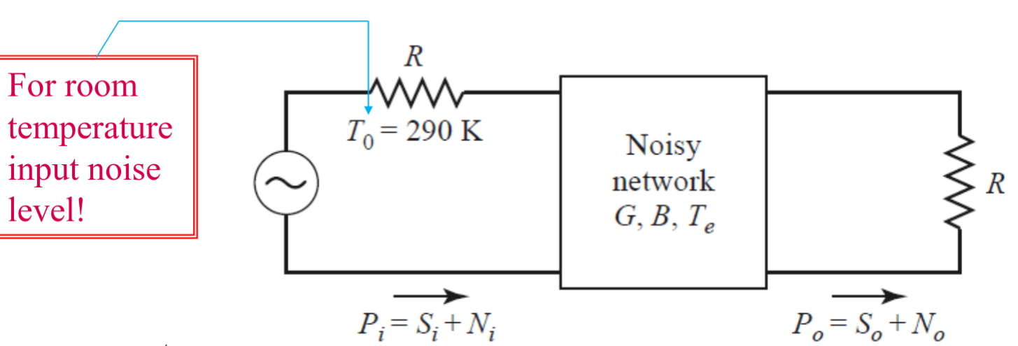
Gain, F and of cascaded system:

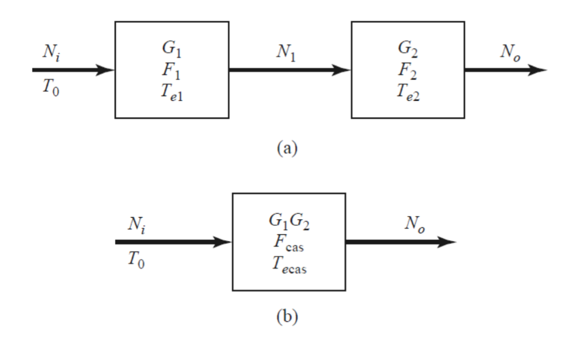
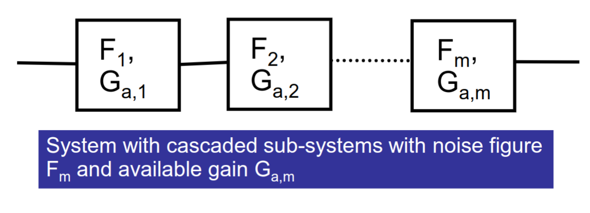
Cascaded NF: Friis’ formula:

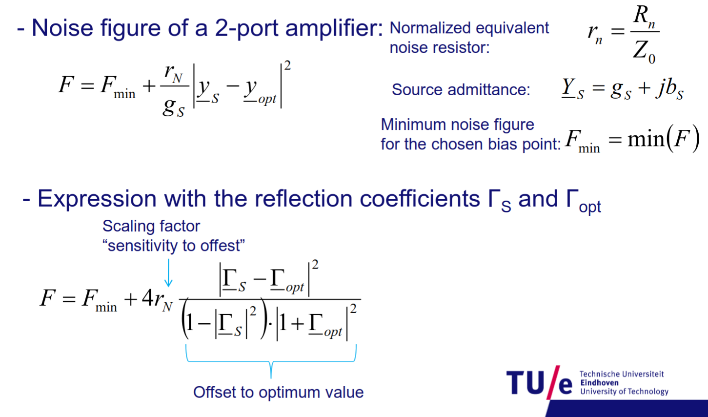
Value of leads to constant val of F.
The values are in circles and we can calculate the center and the radius. The circles are called constant noise circles.


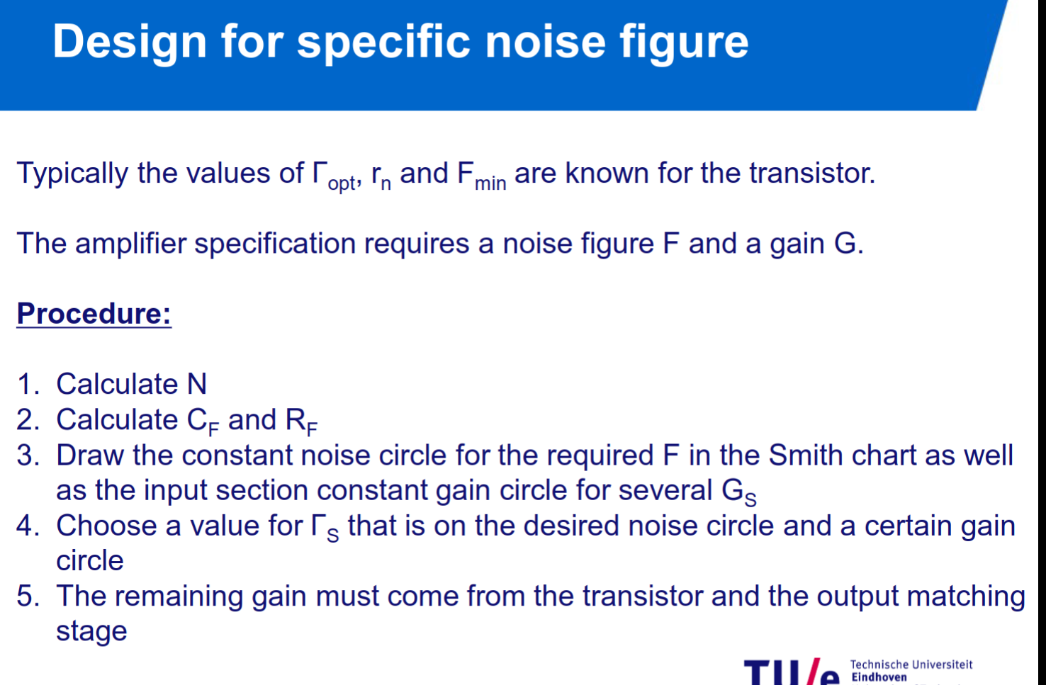
With the Noise figure parameter N defined as:

Basics of PA and Mixer Design (Power amplifiers and mixers)

5XTC0_Module_6_PAs_Mixers (1).pdf

Formulas

Signal-to-noise ratio (SNR):

Thermal noise power:

Noise figure (F):

Noise figure (dB):

Friis’ noise figure formula (cascaded stages):

Noise figure of an amplifier with reflection coefficients:

Noise figure parameter (N):

Constant noise circle radius:

Nonlinear output expression:

1 dB Compression Point: input/output power where gain is reduced by 1 dB from linear response

Second-order intercept point (IIP2): Extrapolated power where second-order products intersect with fundamental

Third-order intercept point (IIP3): Extrapolated input power where third-order products equal fundamental

Cascaded IIP3 formula:

Mixer output signal (RX - time domain):

Intermediate frequency (IF):

Mixer output signal (TX - time domain):

Upconverted frequency (TX):

Mixing in frequency domain:

Output power:

Optimum load resistance:

Maximum PA efficiency (Class A):

System level design

5XTC0_Module7_System_Design.pdf

Formulas

Signal-to-Noise Ratio (SNR)

Friis’ Formula for Cascaded Noise Figure

Cascaded IIP3 Formula

Output Power from Gain

Linear Dynamic Range (LDR)

Spurious Free Dynamic Range (SFDR)

Energy per Bit

Noise Power

Ratio

Receiver Sensitivity (in dBm)

with:

Shannon Capacity

Friis Radio Link Formula (Power at RX input)